Wavetable Synthesis Algorithm Explained

How to generate sound in code using the wavetable synthesis technique?

In this article, you will learn:

• how to generate sound using wave tables,
• step-by-step wavetable synthesis algorithm (also known as fixed-waveform synthesis [7]),
• what are pros and cons of wavetable synthesis, and
• how is wavetable synthesis related to other synthesis methods.

In the follow-up articles, an implementation of this technique in the Python programming language, the JUCE framework, and the Rust programming language are presented.

A Need for a Fast and Efficient Synthesis Method

Computer-based sound synthesis is the art of generating sound through software.

In the early days of digital sound synthesis, sound was synthesised using specialized digital signal processing hardware. Later on, the community started using software for the same purposes but the underlying principles and algorithms remained the same. To obtain real-time performance capabilities with that technology, there was a great need to generate sound efficiently in terms of memory and processing speed. Thus, the wavetable technique was convceived: it is both fast and memory-inexpensive.

From Gesture to Sound

The process of generating sound begins with a musician’s gesture. Let’s put aside who a musician might be or what kind of gestures they perform. For the purpose of this article, a gesture could be as simple as pressing a key on a MIDI keyboard, clicking on a virtual keybord’s key, or pressing a button on any controller device.

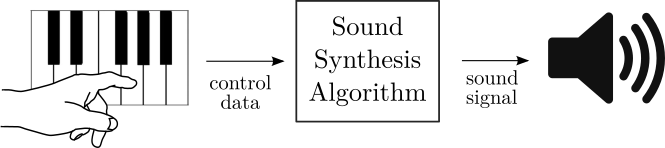Figure 1. In sound synthesis, a gesture of a musician controls the sound generation process.

A gesture provides control information. In the case of pressing a key on a MIDI keyboard, control information would incorporate information on which key was pressed and how fast was it pressed (velocity of a keystroke). We can change the note number information into frequency $f$ and the velocity information into amplitude $A$. This information is sufficient to generate sound using most of the popular synthesis algorithms.

Sine Generator

Let’s imagine that given frequency and amplitude information we want to generate a sine wave. The general formula of a sine waveform is

$s(t) = A \sin (2 \pi f t + \phi), \quad (1)$

where $f$ is the frequency in Hz, $A$ is the amplitude in range $[0, 1]$, $t$ is time in seconds, and $\phi$ is the initial phase, which we will ignore for now (i.e., assume that $\phi=0$).

As we discussed in the digital audio basics article, digital audio operates using samples rather than physical time. The $n$-th sample occurs at time $t$ when

$n = f_s t, \quad (2)$

where $f_s$ is the sampling rate, i.e., the number of samples per second that the system (software or hardware) produces.

After inserting Equation 2 into Equation 1, we obtain the formula for a digital sine wave

$s[n] = A \sin (2 \pi f n / f_s), \quad (3)$

How to compute the $\sin$ in the above formula? In programming languages (and any calculators for that matter), we often have a sin() function, but how does it compute its return value?

sin() calls use the Taylor expansion of the sine function [1]

$\sin(x) = x - \frac{x^3}{3!} + \frac{x^5}{5!} - \frac{x^7}{7!} \dots \quad (4)$

Above expansion is infinite, so on real-world hardware, it needs to be truncated at some point (after obtaining sufficient accuracy). Its advantage is, that it uses operations realizable in hardware (multiplication, division, addition, subtraction). Its disadvantage is that it involves a lot of these operations. If we need to produce 44100 samples per second and want to play a few hundred sines simultaneously (what is typical of additive synthesis), we need to be able to compute the $\sin$ function more efficiently than with Taylor expansion.

A Wave Table

A wave table is an array in memory in which we store a fragment of a waveform. A waveform is a plot of a signal over time. Thus, one period of a sine wave stored in memory looks as follows:

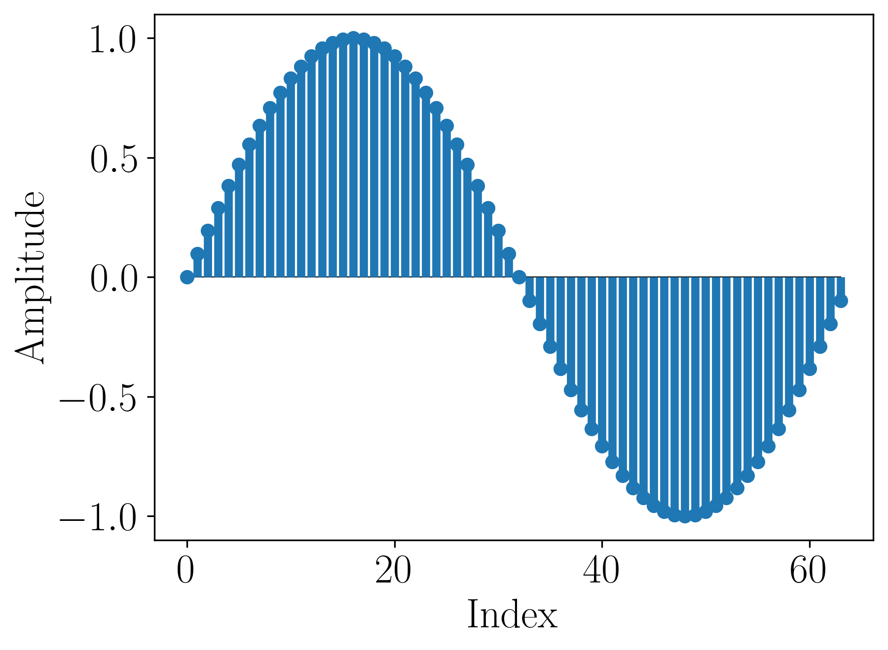Figure 2. A wave table with 64 samples of the sine waveform.

The above wave table uses 64 samples to store one period of the sine wave. These values can be calculated using the Taylor expansion because we compute them only once and store them in memory.

$\sin$ period is exactly $2 \pi$. The period of a wave table is its length, let’s denote it by $L$. For each sample index $k \in \{0, \dots, L-1\}$ in the wave table, there exists a corresponding argument $\theta \in [0, 2\pi)$ of the sine function.

$\frac{k}{L} = \frac{\theta}{2 \pi}. \quad (5)$

The above equation tells us that there is a mapping between the values in the wave table and the values of the original waveform.

Computing a Waveform Value from the Wave Table

Equation 5 holds for $\theta \in [0, 2\pi)$. If we want to calculate the values of arbitrary $x \in \mathbb{R}$, we need to remove the multiplicity of $2 \pi$ contained in $x$ to bring it to the $[0, 2\pi)$ range. In other words, if

$x = 2\pi l + \phi_x, \quad \phi_x \in [0, 2\pi), \quad (6)$

then we want to find $\phi_x$. In software, it can be done by subtracting or adding $2 \pi$ to $x$ until we obtain a value in the desired range. Alternatively, we can use a function called fmod(), which allows us to obtain the remainder of a floating-point division.

We can subsequently compute the corresponding index in the wave table from the proportion in Equation 5.

$k = \frac{\phi_x L}{2\pi}. \quad (7)$

Now waveTable[k] should return the value of $\sin(x)$, right? There is one more step that we need…

What If $k$ Is Non-Integer?

In most cases, $k$ computed in Equation 7 won’t be an integer. It will rather be a floating-point number between some two integers denoting the wave table indices, i.e., $i <= k < i+1, \quad i \in \{0, \dots, L-1\}, k \in [0, L)$.

To make $k$ an integer, we have 3 options:

• truncation (0th-order interpolation): removing the non-integer part of $k$, a.k.a. floor(k),
• rounding: rounding $k$ to $i$ or $i+1$, whichever is nearest, a.k.a. round(k),
• linear interpolation (1st-order interpolation): computing a weighted sum of the wave table values at $i$ and $i+1$. The weights correspond to $k$’s distance to $i+1$ and $i$ respectively, i.e., we return (k-i)*waveTable[i+1] + (i+1 - k)*waveTable[i],
• higher-order interpolation: too expensive and unnecessary for wavetable synthesis.

Each recall of a wave table value is called a wave table lookup.

Wave Table Looping

We know how to efficiently compute a waveform’s value for an arbitrary argument. In theory, given amplitude $A$, frequency $f$, and sampling rate $f_s$, we are able to evaluate Equation 3 for any integer $n$. Using different wave tables, we can obtain different waveforms. It means we can generate an arbitrary waveform at an arbitrary frequency! Now, how to implement it algorithmically?

Thanks to the information on $f$ and $f_s$, we don’t have to calculate the $2 \pi f n / f_s$ argument of $\sin$ in Equation 3 for each $n$ separately. $n$ gets incremented by 1 on a sample-by-sample basis, so as long as $f$ does not change (i.e., we play at a constant pitch), the argument of $\sin$ gets incremented in a predictable manner. Actually, the argument $2 \pi f n / f_s + \phi$ is called the phase of the sine (again, in our considerations $\phi=0$). The difference between the phase of the waveform for neighboring samples is called a phase increment and can be calculated as

$\theta_\text{inc}(f) = 2 \pi f (n+1) / f_s - 2 \pi f n / f_s = 2 \pi f / f_s. \quad (8)$

$\theta_\text{inc}(f)$ depends explicitly on $f$ (tone frequency) and implicitly on $f_s$ (which typically remains unchanged during processing so we can treat it as a constant). With $\theta_\text{inc}(f)$ we can initialize a phase variable to 0 and increment it by $\theta_\text{inc}(f)$ after generating each sample. When a key is pressed we reset phase to 0, calculate $\theta_\text{inc}(f)$ according to the pitch of the pressed key, and start producing the samples.

Index Increment

Having the information on phase increment, we can calculate the index increment, i.e., how the index to the wave table changes with each sample.

$k_\text{inc} = (k+1) - k = \frac{(\phi_x + \theta_\text{inc})L}{2\pi} - \frac{\phi_x L}{2\pi} \\= \frac{\theta_\text{inc} L}{2\pi} = \frac{fL}{f_s}. \quad (9)$

When a key is pressed, we set an index variable to 0. For each sample, we increase the index variable by $k_\text{inc}$ and do a lookup. As long as the key is pressed, $k_\text{inc}$ is nonzero and we perform the wave table lookup.

When index exceeds the wave table size, we need to bring it back to the $[0, L)$ range. In implementation, we can keep subtracting $L$ as long as index is greater or equal to $L$ or we can use the fmod operation. This “index wrap” results from the phase wrap which we discussed below Equation 5; since the signal is periodic, we can shift its phase by the period without changing the resulting signal.

Phase Increment vs Index Increment

Phase increment and index increment are two sides of the same coin. The former has a physical meaning, the latter has an implementational meaning. You can increment the phase and use it to calculate the index or you can increment the index itself. Index increment is more efficient because we don’t need to perform the multiplication by $L$ and the division by $2\pi$ for each sample (Equation 7); we calculate only the increment when the instantaneous frequency changes. We’ll therefore restrict ourselves to the implementations using the index increment.

Wavetable Synthesis Algorithm

Below is a schematic of how wavetable synthesis using index increment works.

Figure 3. A diagram of the wavetable synthesis algorithm using index increment. After [2].

$k_\text{inc}[n]$ is the increment of the index into the wave table. It is denoted as a digital signal because in practice it can be changed on a sample-by-sample basis. It is directly dependent on the frequency of the played sound. If no sound is played $k_\text{inc}[n]$ is 0 and the index should be reset to 0. Alternatively, one could specify that if no sound is played this diagram is inactive (no signals are supplied to or taken from it).

For each new output sample, index increment is added to the index variable stored in a single-sample buffer (denoted by $z^{-1}$ as explained in the article on delays). This index is then “brought back” into the range of wavetable indices $[0, L)$ using the fmod operation. We still keep the fractional part of the index.

Then, we perform the lookup into the wavetable. The lookup can be done using an interpolation strategy of choice.

Finally, we multiply the signal by a sample-dependent amplitude $A[n]$. $A[n]$ signal is called the amplitude envelope. It may be, for example, a constant, i.e., $A[n] = 1, \forall n \in \mathbb{Z}$.

The output signal $y[n]$ is determined by the wave table used for the lookup and currently generated frequency.

We thus created a wavetable synthesizer!

Oscillator

The diagram in Figure 3 presents an oscillator. An oscillator is any unit capable of generating sound. It is typically depicted as a rectangle combined with a half-circle [3, 4] as in Figure 4. That symbol typically has an amplitude input A ($A[n]$ in Figure 3) and a frequency input $f$ (used to calculate $k_\text{inc}[n]$ in Figure 3).

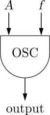Figure 4. The oscillator symbol.

Additionally, what is not shown in Figure 4, an oscillator pictogram usually has some indication of what type of waveform it generates. For example, it may have the sine symbol inside to show that it outputs a sine wave.

Oscillators are sometimes denoted using the VCO abbreviation, which stands for voltage-controlled oscillator. This term originates from the analog days of sound synthesis, when electric voltage determined oscillators’ amplitude and frequency.

Oscillators are the workhorse of sound synthesis. What is presented in Figure 3 is one realization of an oscillator but the oscillator itself is a more general concept. Wavetable synthesis is just one way of implementing an oscillator.

Sound Example: Sine

Let’s use a precomputed wave table with 64 samples of one sine period from Figure 2 to generate 5 seconds of a sine waveform at 440 Hz using 44100 Hz sampling rate.

We thus have $L = 64$, $f=440$ Hz, $f_s=44100$ Hz, $k_\text{inc} = 0.6395\dots$. The resulting sound is:

The magnitude spectrum of this tone is shown below.

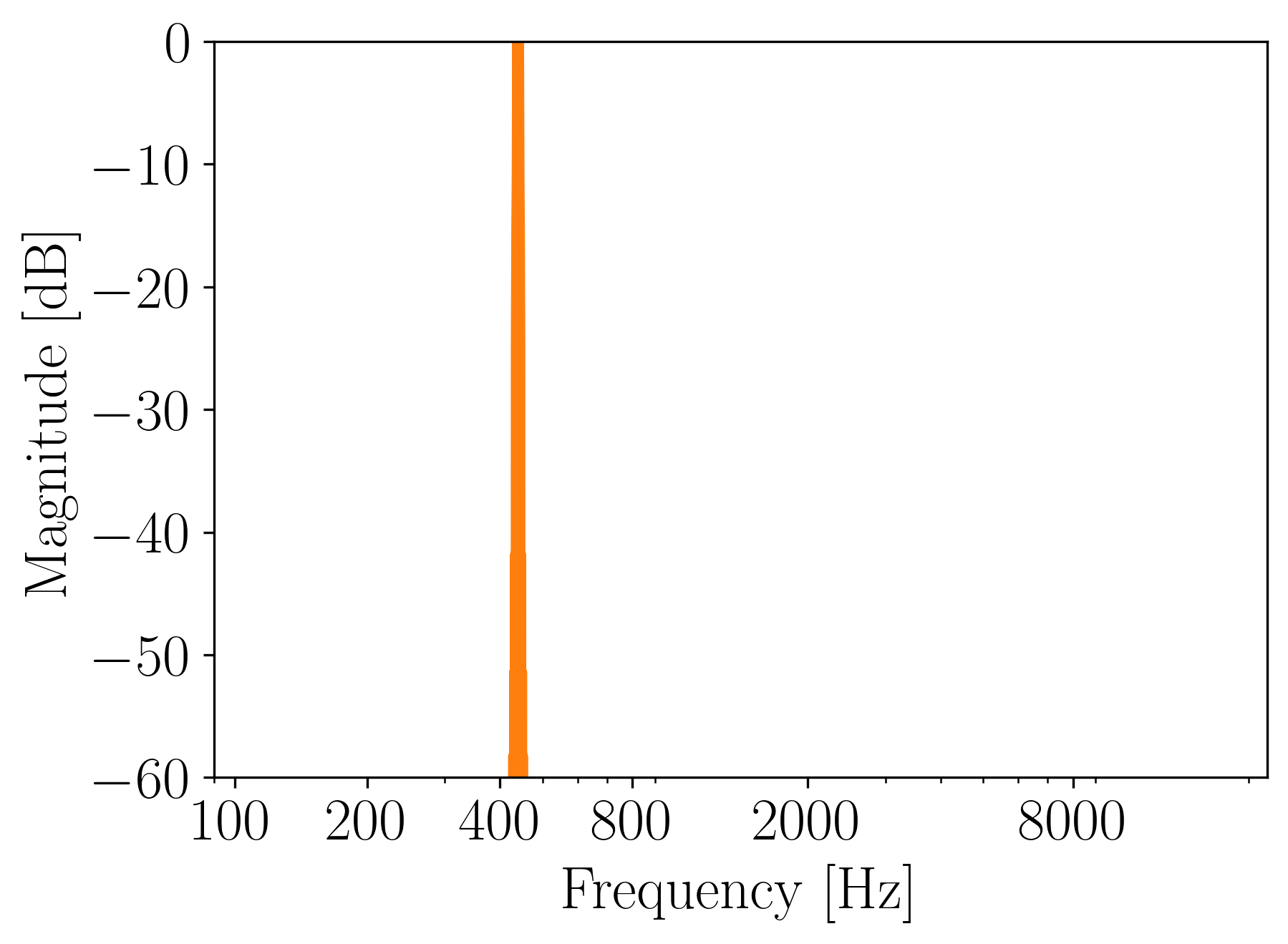Figure 5. Magnitude frequency spectrum of a sine generated with wavetable synthesis.

Great! It sounds like a sine and we obtain just one frequency component. Everything as expected! Now, let’s generate sound using a different wavetable, shall we?

Sound Example: Sawtooth

To generate a sawtooth, we use the same parameters as before just a different wave table:

Figure 6. A wave table with 64 samples of the sawtooth waveform.

Let’s listen to the output:

That sounds ok, but we hear some ringing. How does it look in the spectrum?

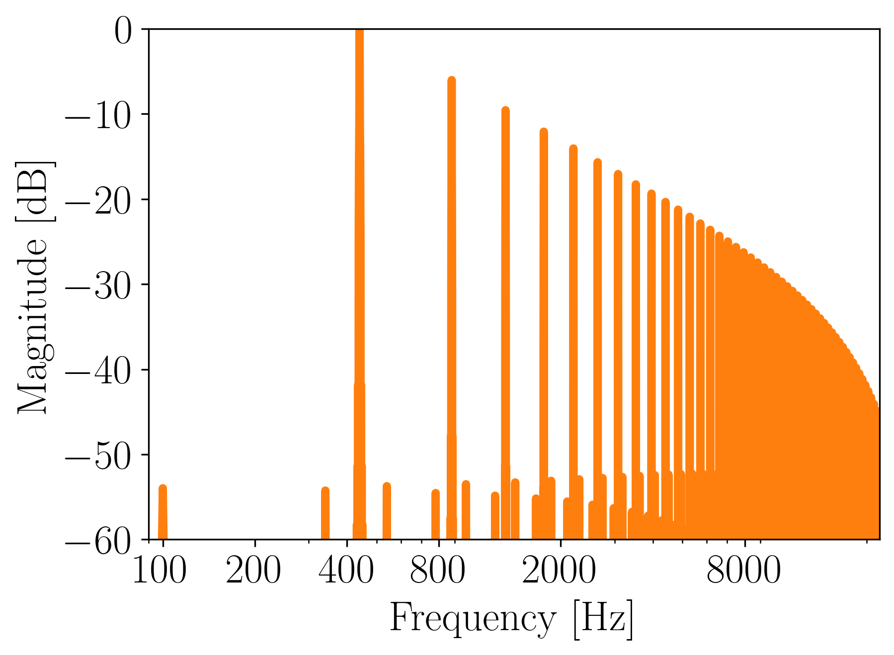Figure 7. Magnitude frequency spectrum of a sawtooth generated with wavetable synthesis.

We can notice that there are some inharmonic frequency components that do not correspond to the typical decay of the sawtooth spectrum. These are aliased partials which occur because the spectrum of the sawtooth crossed the Nyquist frequency. To learn more about why this happens, you can check out my article on aliasing.

Aliasing increases if we go 1 octave higher:

Ouch, that doesn’t sound nice. The frequency spectrum reveals aliased partials that appear as inharmonicities:

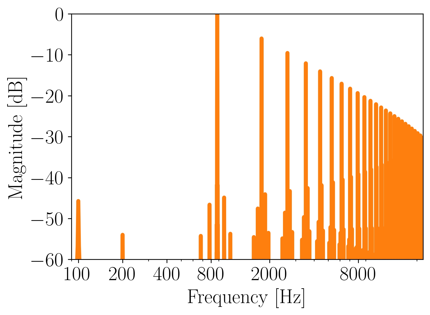Figure 8. Magnitude frequency spectrum of a 880Hz sawtooth generated with wavetable synthesis.

We’ve just discovered the main drawback of wavetable synthesis: aliasing at high frequencies. If we went even higher with the pitch, we would obtain a completely distorted signal.

How to fix aliasing for harmonic-rich waveforms? We can only increase the sampling rate of the system. Since it is not something we would like to do, pure wavetable synthesis is rarely used nowadays.

The type of digital distortion seen in Figure 8 was typical of the early digital synthesizers of the 1980s. A lot of effort was put into the development of alternative algorithms to synthesize sound. The main focus was to obtain an algorithm that would produce partial-rich waveforms at low frequencies and partial-poor waveforms at high frequencies. These algorithms are sometimes called antialiasing oscillators. An example of such an oscillator can be found in “Oscillator and Filter Algorithms for Virtual Analog Synthesis” paper by Vesa Välimäki and Antti Huovilainen [5].

Abstract Waveforms

With wavetable synthesis we can use arbitrary wavetables. For example, in Figure 9, I summed 5 Gaussians, subtracted the mean and introduced a fade-in and fade-out.

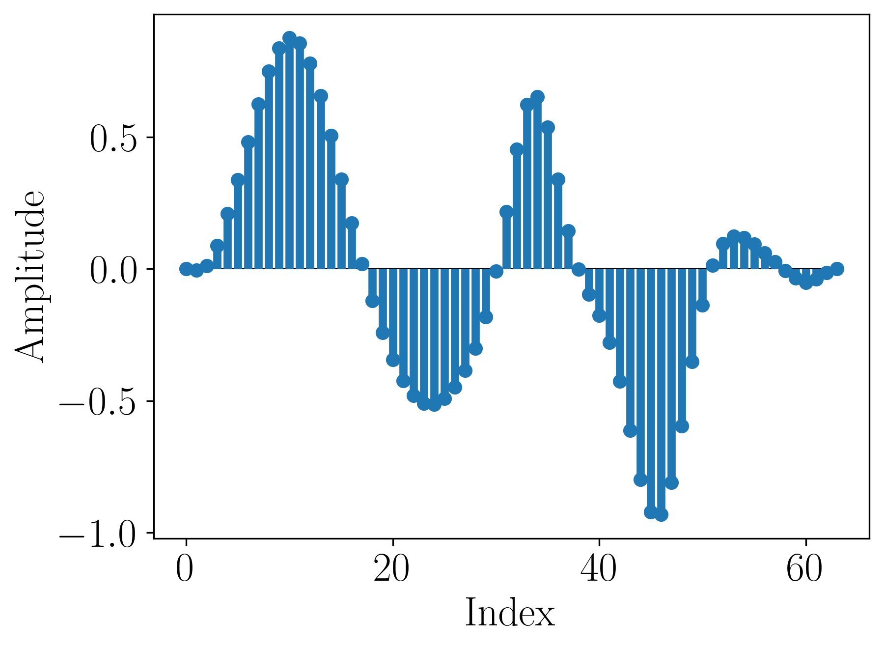Figure 9. An abstract wave table constructed with 5 Gaussians.

Here is a sound generated using this wave table at 110 Hz.

Sounds like a horn, doesn’t it?

Here’s its spectrum:

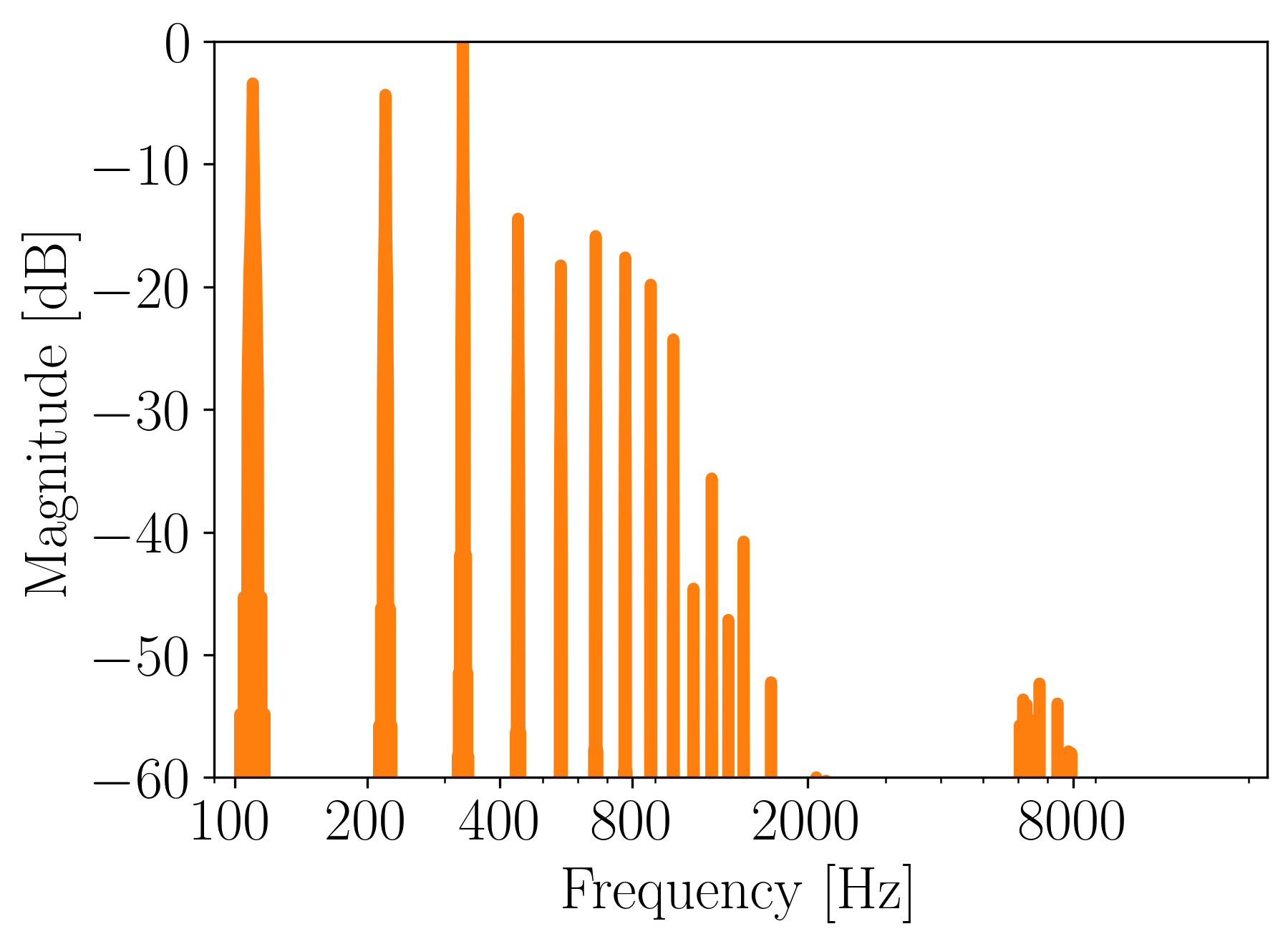Figure 10. Magnitude frequency spectrum of a 110 Hz sound generated from an abstract wavetable.

As we can see, it decays quite nicely, so no audible aliasing is present.

Sampling: Extended Wavetable Synthesis?

Sampling is a technique of recording real-world instruments and playing back these sounds according to user input. We could, for example, record single guitar notes with pitches corresponding to all keys on the piano keyboard. In practice, however, notes for only some of the keys are recorded and the notes in between are interpolated versions of its neighbors. In this way, we store separate samples for high-pitched notes and thus avoid the problem of aliasing because it’s not present in the data in the first place.

Wavetable synthesis could be viewed as sampling with the samples truncated to one waveform period [4].

With sampling, a lot more implementation issues come up. Since sampling is not the topic of this article, we won’t discuss it here.

Single-Cycle, Multi-Cycle, and Multiple Wavetable

What we discussed so far is a single-cycle variant of the wavetable synthesis, where we use just 1 period of a waveform stored in memory to generate the sound (Figure 11). There are more options available.

Figure 11. Single-cycle wavetable synthesis loops over 1 wave table.

In multi-cycle wavetable synthesis, we effectively concatenate different wavetables, whose order can be fixed or random (Figure 12).

Figure 12. Multi-cycle wavetable synthesis loops over multiple wave tables, possibly in a cycle.

For example, we could concatenate sine, square, and sawtooth wave tables to obtain a more interesting timbre.

The resulting wave table would look like this:

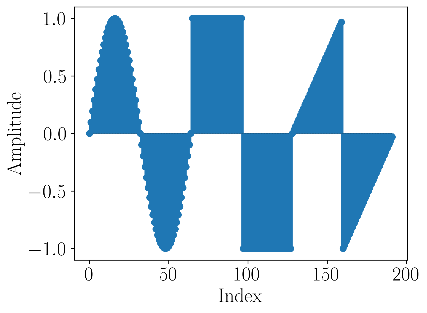Figure 13. A wave table from a concatenation of sine, square, and sawtooth wave tables.

Here is a sound generated using this wave table at 330 Hz.

One can hear the characteristics of all 3 waveforms.

Here’s its spectrum:

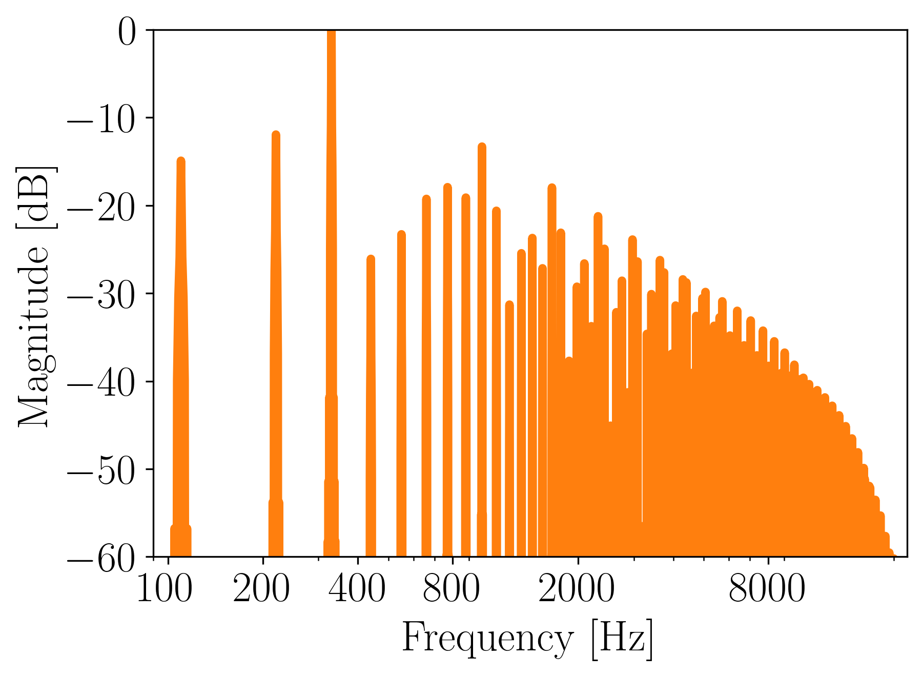Figure 14. Magnitude frequency spectrum of a 330 Hz sound generated from a concatenation of wave tables.

The above spectrum is heavily aliased. Additionally, we got a frequency component at 110 Hz. That is because by concatenating 3 wave tables, we essentially lengthened the base period of the waveform, effectively lowering its fundamental frequency 3 times. Original waveform was at 330 Hz; the fundamental is now at 110 Hz.

In multiple wavetable variant, one mixes a few wave tables at the same time (Figure 15).

Figure 15. Multiple wavetable synthesis mixes between multiple wave tables while looping over them.

The impact of each of the used wave tables may depend on control parameters. For example, if we press a key mildly, we can get a sine-like timbre, but if we press it fast, we may hear more high-frequency partials. That could be realized by mixing the sine and sawtooth wave tables. The ratio of these waveforms would directly depend on the velocity of the key stroke. There could also be some gradual change in the ratio while a key is pressed.

Summary

Wavetable synthesis is an efficient method that allows us to generate arbitrary waveforms at arbitrary frequencies. Its low complexity comes at a cost of high amounts of digital distortion caused by the harmonics crossing the Nyquist frequency at high pitches.

Pros of wavetable synthesis:

• computational efficiency,
• direct frequency-to-parameters mapping,
• arbitrary waveform generation.

Cons of wavetable synthesis:

• aliasing already at moderately high frequencies,
• requires further processing and/or extensions to be musically interesting.

Software synthesizers typically use more sophisticated algorithms than the one presented in this article. Nevertheless, wavetable synthesis underlies many other synthesis methods. The produced waveform could be further transformed. Therefore, the discussion of wavetable synthesis allows us to understand the basic principles of digital sound synthesis.

Bibliography

These are the references I used for this article. If you are interested in the topic of sound synthesis, each of them is a valuable source of information. Alternatively, subscribe to WolfSound’s newsletter to stay up to date with the newly published articles on sound synthesis!

[1] Taylor series expansion of the sine function on MIT Open CourseWare

[2] F. Richard Moore, Elements of Computer Music, Prentice Hall 1990

[3] Curtis Roads, Computer Music Tutorial, MIT Press 1996

[4] Marek Pluta, Sound Synthesis for Music Reproduction and Performance, monograph, AGH University of Science and Technology Press 2019.

[5] Vesa Välimäki and Antti Huovilainen, Oscillator and Filter Algorithms for Virtual Analog Synthesis, Computer Music Journal 30(2):19-31, June 2006

[6] Martin Russ, Sound Synthesis and Sampling, 3rd Edition, Focal Press, 2009.

[7] Giovanni De Poli, A Tutorial on Digital Sound Synthesis Techniques, Computer Music Journal, January 1992.

Links above may be affiliate links. That means that I may earn a commission if you decide to make a purchase. This does not incur any cost for you. Thank you.