Convolution: The secret behind filtering

Why does filtering work? What enables us to enhance the bass in our audio players?

Please accept marketing cookies to access the video player.

There is one operation that stands behind it all: convolution.

In order to fully master filtering, be it finite impulse response (FIR) or infinite impulse response (IIR) filtering, one needs to understand the definition, derivation and the properties of the convolution operation very well. That will be the topic of this and a few following articles.

We are going to dig deep into the convolution and we will get to know it so well, that it won’t surprise us any more and we’ll be able to recognize it from afar.

This article outlines the mathematical definition of the convolution and gives you some intuition behind it. In the next article we will introduce some basic properties along with their proofs (told you it’s going to go deep).

Are you ready?

The Convolution Series

Definition of convolution and intuition behind it
Mathematical properties of convolution
Convolution property of Fourier, Laplace, and z-transforms
Identity element of the convolution
Star notation of the convolution
Circular vs. linear convolution
Fast convolution
Convolution vs. correlation
Convolution in MATLAB, NumPy, and SciPy
Deconvolution: Inverse convolution
Convolution in probability: Sum of independent random variables

Definition

In its simplest form, the convolution between two discrete-time signals $x[n]$ and $h[n]$ can be expressed as an infinite sum

x[n] \ast h[n] = \sum_{k=-\infty}^{\infty} x[k] h[n - k] = y[n], \quad n \in \mathbb{Z}. \quad (1)

Whoa, what’s happened here? Under the sum we have the two signals, but the second one is not only shifted in time by $n$ but also time-reversed!

Important assumptions

In order to make this discussion feasible, we must enforce $x[n]$ and $h[n]$ to have finite energy. A signal $s[n]$ is said to have finite energy, if

\sum_{n=-\infty}^{\infty} s^2[n] < \infty, \quad (2)

i. e., $s[n]$ is square-summable.

Additionally, we also assume that all considered signals $s[n]$ ( $x[n], h[n], y[n]$ , etc.) are 0 for negative time indices, i. e., $s[n] = 0 \quad \forall n < 0$ .

Intuition

In order to get an intuition behind the convolution, we should look at it from different perspectives.

Filtering perspective

Let’s consider a generic filter with input $x[n]$ , output $y[n]$ , and impulse response $h[n]$ (Figure 1).

Figure 1. A generic filter.

A filter is a linear time-invariant (LTI) system. From signal processing we know that any LTI system is completely specified by its impulse response $h[n]$ . The output $y[n]$ of an LTI system is by definition equal to the convolution of the input $x[n]$ with the system’s impulse response $h[n]$ . That is why the output of an LTI system is called a convolution sum or a superposition sum in case of discrete systems and a convolution integral or a superposition integral in case of continuous systems.

Now, let’s consider again Equation 1 with $h[n]$ denoting the filter’s impulse response and $x[n]$ denoting the filter’s input signal. We may look at the filter’s output $y[n]$ as a weighted sum of filter’s impulse responses. How?

Consider $n=0$ . At the output we get

y[0] = \sum_{k=-\infty}^{\infty} x[k] h[0 - k] = \sum_{k=-\infty}^{\infty} x[k] h[- k] = x[0] h[0],

y[1] = \sum_{k=-\infty}^{\infty} x[k] h[1 - k] = x[0]h[1] + x[1]h[0].

Delaying-and-summing perspective

We can also look at that operation from a different perspective. What if we fix $k$ in Equation 1? In this case, it describes the output of the system if only input sample $x[k]$ was given:

y_k[n] = x[k]h[n-k]. \quad (3)

The above equation basically says, that once $x[k]$ enters the filter, it will weigh its entire impulse response delayed by $k$ samples with respect to $n$ . We then just have to sum up over all possible $k$ values to conclude that $y[n]$ is just filter’s impulse response, delayed and weighted by each sample of $x[n]$ .

This may all get a little bit confusing at this moment, so let’s look at an example, shall we?

Example

Let’s consider the following signal $x[n]$ of length 4, i. e., consisting of $x[0], x[1], x[2]$ , and $x[3]$

Figure 2. Input signal $x[n]$ .

and filter’s impulse response $h[n]$ of length 3

Figure 3. Filter’s impulse response $h[n]$ .

The result of their convolution is the following signal $y[n]$ (filter’s output)

Figure 4. Filter’s output $y[n]$ after feeding $x[n]$ at the input.

Not very meaningful, is it? The only thing that we can observe is that output’s length is the sum of input’s and filter’s lengths minus one.

Let’s try some color coding. We can depict each of $x[n]$ 's samples in a different color:

Figure 5. Color-coded $x[n]$ .

We can now examine the impact of particular samples on the filter’s output. What would happen if only blue $x[0]$ entered the filter?

Figure 6. Filter’s response to $x[0]$ .

We can see that the entire impulse response of the filter got scaled by $x[0]$ which in this case is equal to $0.1$ .

Now, let’s imagine, that only second sample, namely orange $x[1]$ , entered the filter. What could we observe at the output?

Figure 7. Filter’s response to $x[1]$ .

Notice that at $n=0$ the filter’s output is $0$ , because at that time $x[1]$ has not yet entered the filter. But from $n=1$ onwards we get again the filter’s impulse response scaled by the newly entering sample.

The same thing happens for green $x[2]$ and red $x[3]$ Figure 8. Filter’s response to 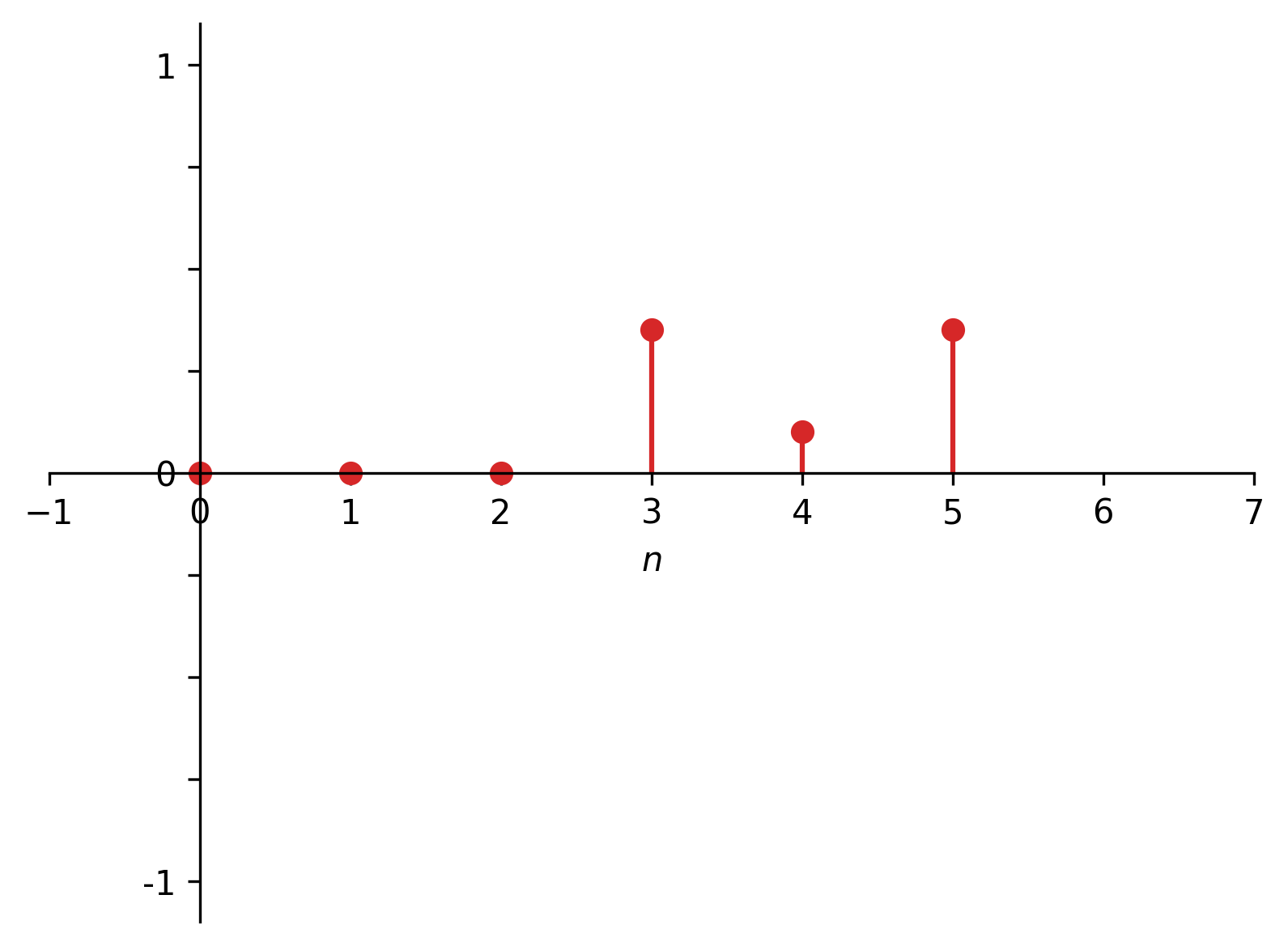$x[2]$ . Figure 9. Filter’s response to $x[3]$ .

Viewing all these “partial” responses on a plot shows the impact of each individual input sample over time Figure 10. Overlayed filter’s responses to individual samples of $x[n]$ .

Summing them all up (as if summing over $k$ in the convolution formula) we obtain: Figure 11. Summation of signals in Figures 6-9. what corresponds to the $y[n]$ signal above.

Continuous convolution

Convolution is defined for continuous-time signals as well (notice the conventional use of round brackets for non-discrete functions)

x(t) \ast h(t) = \int \limits_{-\infty}^{\infty} x(\tau) h(t - \tau) d\tau. \quad (4)

Although it may not be as intuitive in interpretation as the discrete convolution, nevertheless, we could try to imagine the continuous case as an infinitely densely sampled discrete signal (so that the sum over discrete samples changes to an integral over continuous functions). But keep in mind that it is only an intuitive view not a mathematically strict interpretation.

Summary

In this article, we introduced the mathematical operation of convolution, gave the justification for its form, and provided a little bit of intuition on how can we view the convolution from different angles. In the next articles we are going to study convolution more closely.

Up next: mathematical properties of convolution!.

Bibliography

[1] Convolution on Wikipedia. Retrieved: 09.03.2021.

[2] Alan V Oppenheim, Ronald W. Schafer Discrete-Time Signal Processing, 3rd Edition, Pearson 2010.

[3] Alan V. Oppenheim, Alan S. Willsky, with S. Hamid Signals and Systems, 2nd Edition, Pearson 1997.

Please accept marketing cookies to access the display and add comments.