Fast Convolution: FFT-based, Overlap-Add, Overlap-Save, Partitioned

How to compute convolution fast for real-time applications?

Please accept marketing cookies to access the video player.

The Convolution Series

Introduction

Sound engineering and Virtual Reality audio demand real-time performance. Convolutions are inherently embedded in their inner workings, e.g., in the form of finite impulse response (FIR) filtering for artificial reverberation. Convolution evaluated according to the definition is too slow to keep up and introduces audible latency. To mitigate this we reach out to the fast convolution methods.

But speed itself is not enough. In the above-mentioned applications we need to process sound in a block-wise fashion. Methods allowing this are called partitioned convolution techniques.

In this article, we first show why the naive approach to the convolution is inefficient, then show the FFT-based fast convolution. What follows is a description of two of the most popular block-based convolution methods: overlap-add and overlap-save. Finally, we show how to deal with very long filters (over 1 second long) when using partitioned convolution.

Note: An amazing source about fast convolution techniques is [1]. I highly encourage you to check it out especially if you would like to read more on the topic.

Notation

In software, the signals are always of finite length. Thus, we will denote a signal $x[n]$ of length $N_x$ by a fixed-size vector $\pmb{x} = [x[0], x[1], \dots, x[N_x-1]]$ .

Naive implementation of convolution

We could implement the convolution between discrete-time signals $x$ and $h$ by implementing the definition directly [1]

y[n] = x[n] \ast h[n] = \sum_{k=\max\{0,n-N_h+1\}}^{\min\{n, N_x-1\}} x[k] h[n - k], \newline \quad n \in \{0, \dots, N_x + N_h - 1\}. \quad (1)

This translates to the following code

def naive_convolution(x, h):    
    """Compute the discrete convolution of two sequences"""
    
    # Make x correspond to the longer signal
    if len(x) < len(h):
        x, h = h, x
        
    M = len(x)
    N = len(h)
    
    # Convenience transformations
    x = pad_zeros_to(x, M+2*(N-1))
    x = np.roll(x, N-1)
    
    h = np.flip(h)
    
    y = np.zeros(M+N-1)

    # Delay h and calculate the inner product with the 
    # corresponding samples in x
    for i in range(len(y)):
        y[i] = x[i:i+N].dot(h)
        
    return y

Listing 1. Naive linear convolution.

FFT-based implementation

As we know from the article on circular convolution, multiplication in the discrete-frequency domain is equivalent to circular convolution in the discrete-time domain. Element-wise multiplication of 2 vectors has time complexity $O(N)$ . This is superior to $O(N^2)$ in case of the naive approach. The bottleneck of frequency-based convolution is the transformation to that domain, but it can be achieved in $O(N \log N)$ time, which is still better than $O(N^2)$ . And so arises the FFT-based fast convolution (Figure 1).

Figure 1. FFT-based fast convolution. Source: [1].

In order to make circular convolution correspond to linear convolution we need to pad the input signals with sufficiently many zeros so that the frequency-domain representation has enough capacity to represent the result of the linear convolution. This means, that each signal should be extended to have length $K = Nx + Nh - 1$ .

We can obtain it using function pad_zeros_to().

def pad_zeros_to(x, new_length):
    """Append new_length - x.shape[0] zeros to x's end via copy."""
    output = np.zeros((new_length,))
    output[:x.shape[0]] = x
    return output

Listing 2.

If our signals are sufficiently long we can compute their discrete Fourier transforms (DFTs) using the Fast Fourier Transform (FFT) algorithm. Thanks to the FFT, the transformation from the time domain to the frequency domain can be computed in $O(N \log N)$ time.

In the frequency domain we can multiply our signals element-wise and then come back to the time domain via inverse FFT.

FFT is known to be most computationally efficient if the transformed signal’s length is a power of 2. We can compute the exponent of the next largest power of 2 with respect to an integer $n > 0$ using the formula

q_{\text{next}} = \log2(n - 1) + 1. \quad (2)

The above equation allows us to implement another helper function

def next_power_of_2(n):
    return 1 << (int(np.log2(n - 1)) + 1)

Listing 3.

Wrapping it all together

def fft_convolution(x, h, K=None):
    Nx = x.shape[0]
    Nh = h.shape[0]
    Ny = Nx + Nh - 1 # output length

    # Make K smallest optimal
    if K is None:
        K = next_power_of_2(Ny)

    # Calculate the fast Fourier transforms 
    # of the time-domain signals
    X = np.fft.fft(pad_zeros_to(x, K))
    H = np.fft.fft(pad_zeros_to(h, K))

    # Perform circular convolution in the frequency domain
    Y = np.multiply(X, H)

    # Go back to time domain
    y = np.real(np.fft.ifft(Y))

    # Trim the signal to the expected length
    return y[:Ny]

Listing 4. FFT-based fast convolution.

Remember that the above algorithm is fast algorithmically. I am not claiming this code is maximally optimized 😉. It is provided for understanding and as a possible baseline implementation.

Block-based convolution

FFT-based fast convolution is sufficiently fast for offline computation, but musical and virtual reality applications require real-time performance. In these applications, sound is usually processed in blocks of length 64, 128, 256, or more samples. If the signals to be convolved are longer than the block length, we need to adapt our methods so that we can convolve and output only partial results and handle incoming input.

In this section, we will assume that the input signal is an infinite stream (e.g., a looped source replaying a sound file) that comes in blocks $\pmb{x}$ of $B$ samples, and $\pmb{h}$ is a FIR filter of length $N$ . Such a set-up is called unified input partitioning because the input comes in blocks and the blocks are of equal size.

Overlap-Add Scheme

The first idea to process the input in blocks is to convolve each incoming block with the full filter using FFT-based convolution, store the results of appropriately many past convolutions, and output sums of their subsequent parts in blocks of the same length as the input signal we process. This scheme can be seen in Figure 2.

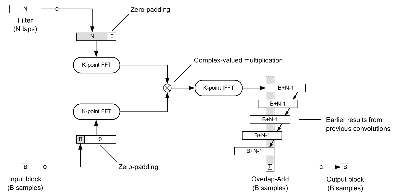Figure 2. Overlap-Add convolution scheme. Source: [1].

Some important remarks concerning this methodology:

$K$ (transform length) must be sufficiently large to ensure that the circular convolution is equivalent to the linear convolution (no samples are time-aliased). Lengthening the convolved signals is achieved through zero-padding.
Overlap-Add operation to form the output block is much more difficult than it may seem from the scheme. One needs to store all the convolution results and then sum appropriate indices. This may incur high memory and time cost.

Implementation

def overlap_add_convolution(x, h, B, K=None):
    """Overlap-Add convolution of x and h with block length B"""

    M = len(x)
    N = len(h)

    # Calculate the number of input blocks
    num_input_blocks = np.ceil(M / B).astype(int)

    # Pad x to an integer multiple of B
    xp = pad_zeros_to(x, num_input_blocks*B)

    # Your turn ...
    output_size = num_input_blocks * B + N - 1
    y = np.zeros((output_size,))
    
    # Convolve all blocks
    for n in range(num_input_blocks):
        # Extract the n-th input block
        xb = xp[n*B:(n+1)*B]

        # Fast convolution
        u = fft_convolution(xb, h, K)

        # Overlap-Add the partial convolution result
        y[n*B:n*B+len(u)] += u

    return y[:M+N-1]

Listing 5. Overlap-Add convolution.

Overlap-Save Scheme

A significant drawback of the Overlap-Add scheme is the necessity to store and sum the computed partial convolutions. Can we do better?

Another approach is called Overlap-Save. It is based on storing appropriately many input blocks rather than output blocks, which are shorter than the calculated convolutions. The input blocks are stored in a buffer of length $K$ in a First-In-First-Out manner, i.e., each new block of input samples shifts all previously stored samples in the buffer, discarding the oldest $B$ samples. We then perform a $K$ -point FFT-based convolution with the zero-padded filter coefficients.

Inherently, the result of this operation is a circular convolution (because the input signal is not zero-padded). It means that $K$ has to be sufficiently large so as to have the last $B$ samples correspond to the linear convolution. We can then output these $B$ valid samples and discard the rest. This results in a potentially longer transform length than in the Overlap-Add scheme, but removes the need to store and sum the outputs.

The entire scheme can be seen in Figure 3.

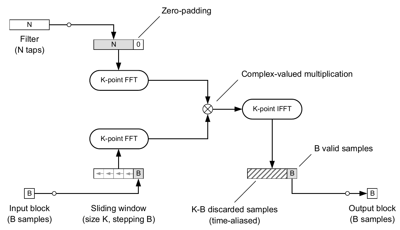Figure 3. Overlap-Save convolution scheme. Source: [1].

Implementation

def overlap_save_convolution(x, h, B, K=None):
    """Overlap-Save convolution of x and h with block length B"""

    M = len(x)
    N = len(h)

    if K is None:
        K = max(B, next_power_of_2(N))
        
    # Calculate the number of input blocks
    num_input_blocks = np.ceil(M / B).astype(int) \
                     + np.ceil(K / B).astype(int) - 1

    # Pad x to an integer multiple of B
    xp = pad_zeros_to(x, num_input_blocks*B)

    output_size = num_input_blocks * B + N - 1
    y = np.zeros((output_size,))
    
    # Input buffer
    xw = np.zeros((K,))

    # Convolve all blocks
    for n in range(num_input_blocks):
        # Extract the n-th input block
        xb = xp[n*B:n*B+B]

        # Sliding window of the input
        xw = np.roll(xw, -B)
        xw[-B:] = xb

        # Fast convolution
        u = fft_convolution(xw, h, K)

        # Save the valid output samples
        y[n*B:n*B+B] = u[-B:]

    return y[:M+N-1]

Listing 6. Overlap-Save convolution.

What If the Filter Is Long Too?

If the filter we want to convolve the input with has also significant length (e.g., when it represents an impulse response of a large hall with a significant reverberation time), we may have to partition both, the input and the filter. These methods are called partitioned convolution.

Describing partitioned convolution algorithms is beyond the scope of this article, but the main idea is presented in Figure 4. It shows a non-uniformly partitioned convolution scheme, which is generally faster than uniformly partitioned versions [1]. It also involves the use of frequency-domain delay lines (FDLs), which allow computing the FFT of the input blocks just once (in contrast to time-delaying the input blocks and calculating their FFTs for each new output block).

Non-uniformly partitioned convolution is the current state of the art in artificial reverberation using FIR filters for real-time auralization in games and Virtual Reality.

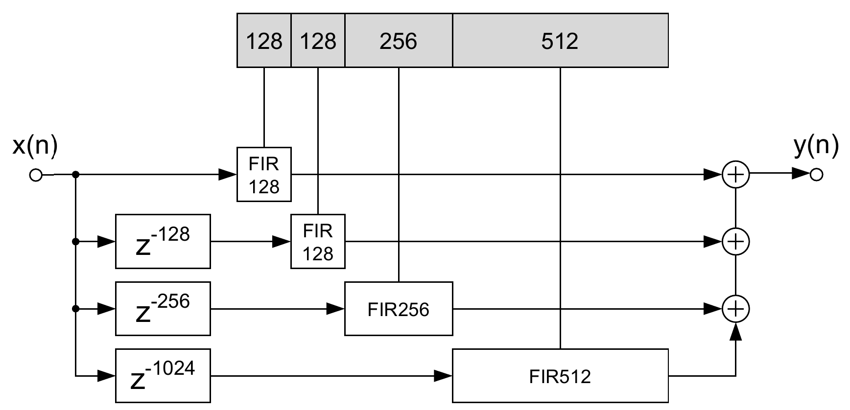Figure 4. Non-uniformly partitioned convolution scheme. Note the presence of frequency-domain delay lines. Source: [1].

Summary

In this article, we have reviewed the most important convolution algorithms:

naive linear convolution of fixed-length signals,
FFT-based convolution of fixed-length signals,
Overlap-Add and Overlap-Save block-based convolution schemes with unified input partitioning, where the input comes in blocks and the filter is of finite, short length, and
Non-uniformly partitioned convolution where the input comes in blocks and the filter is very long.

With an understanding of these concepts you can rush off to code an unforgettable sonic Virtual Reality experience!

Bibliography

[1] Frank Wefers Partitioned convolution algorithms for real-time auralization, PhD Thesis, Zugl.: Aachen, Techn. Hochsch., 2015.

Please accept marketing cookies to access the display and add comments.

Fast Convolution: FFT-based, Overlap-Add, Overlap-Save, Partitioned

The Convolution Series

Introduction

Notation

Naive implementation of convolution

FFT-based implementation

Block-based convolution

Overlap-Add Scheme

Implementation

Overlap-Save Scheme

Implementation

What If the Filter Is Long Too?

Summary

Bibliography

Welcome to WolfSound!

W

TR