Can we calculate correlation using convolution?
The Convolution Series
- Definition of convolution and intuition behind it
- Mathematical properties of convolution
- Convolution property of Fourier, Laplace, and z-transforms
- Identity element of the convolution
- Star notation of the convolution
- Circular vs. linear convolution
- Fast convolution
- Convolution vs. correlation
- Convolution in MATLAB, NumPy, and SciPy
- Deconvolution: Inverse convolution
- Convolution in probability: Sum of independent random variables
In many contexts, convolution and correlation are mixed up. One of the biggest sources of this confusion is deep learning, where convolutional neural networks are often implemented using discrete correlation rather than discrete convolution. That is possible, because the order of elements in the convolution masks does not matter: it can be simply learned as flipped [3].
Let’s explain the difference between correlation and convolution once and for all.
Convolution Definition
Continuous convolution is defined as
Discrete convolution is defined as
Click here to read about the rationale behind these formulas.
Correlation Definition
Correlation is a notion from the field of stochastic processes. In signal processing we simply use an entity called the correlation function [1]
Analogously, we have a correlation function for real-valued discrete-time signals [1]
Sometimes
In the subsequent discussion, we assume that the integrals in Equations 1 and 3, and sums in Equations 2 and 4 converge.
Example
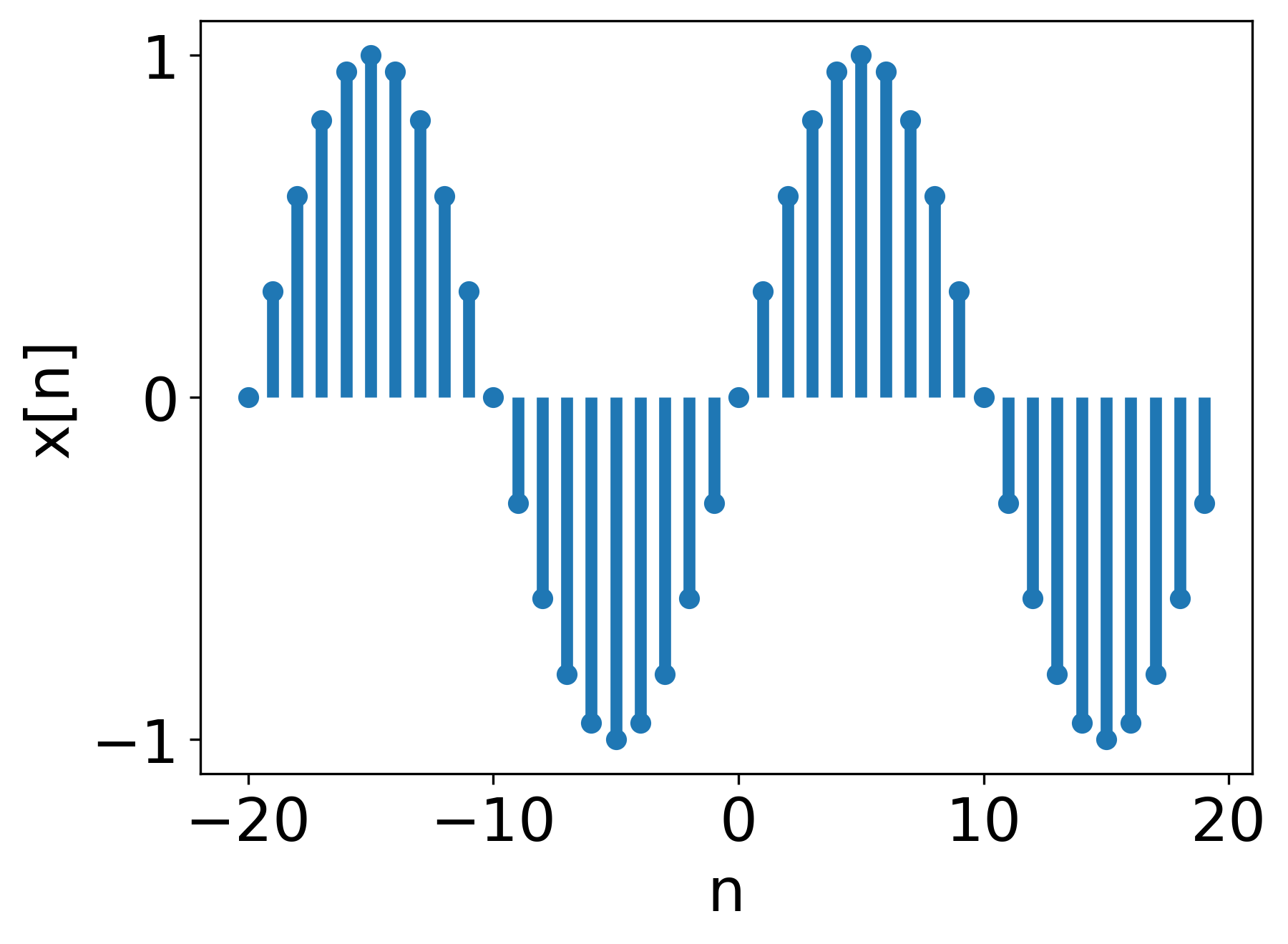
Let’s assume we have two signals of length 40,
 Figure 1.
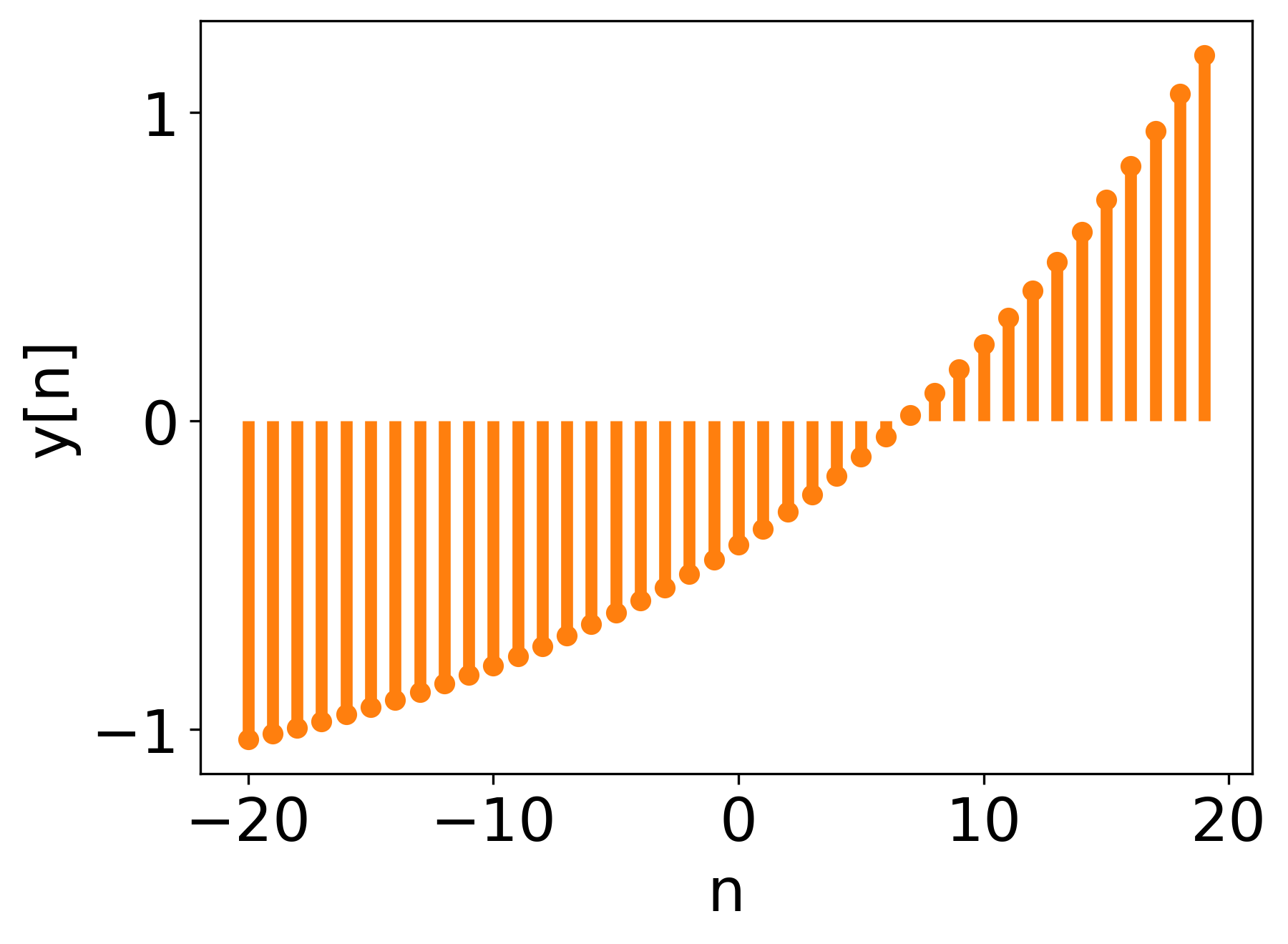
and
 Figure 2.
The convolution between
 Figure 3. Convolution of
and their correlation in Figure 4.
 Figure 4. Correlation of
As you can observe, they are kind of similar.
Correlation as a Similarity Measure
In the context of signal processing, correlation is interpreted as a similarity measure, i.e., how similar are the two correlated signals for a specific lag in samples (relative shift between the signals).
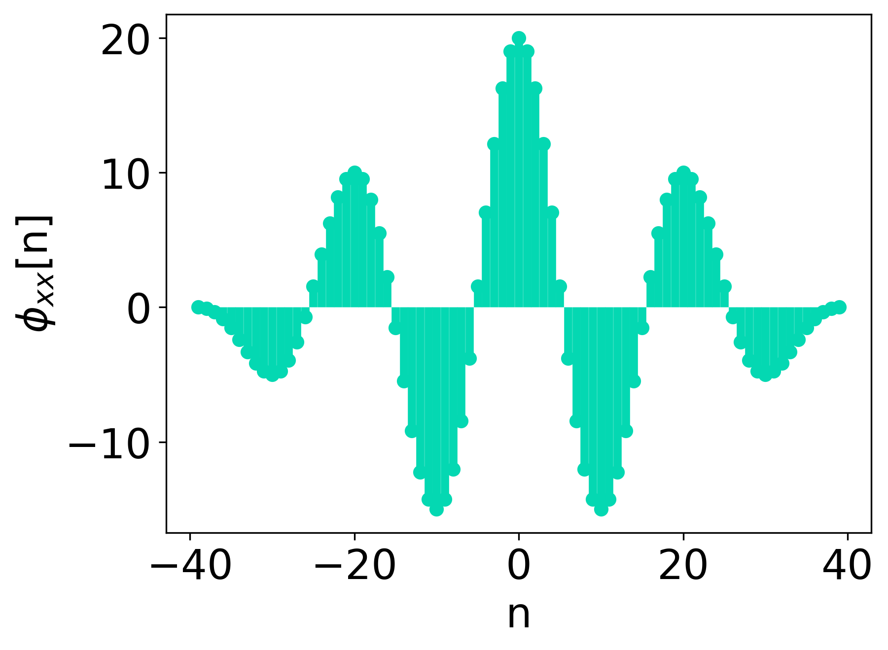
This concept is best visibile for autocorrelation, which is a measure of self-similarity.
In Figure 5, we can see the autocorrelation of signal
 Figure 5. Autocorrelation of
Obviously, autocorrelation achieves its peak value for lag
However, two clear maxima can be observed for relative shifts of
As you can see, autocorrelation can help us determine the periodicity of a signal. This property is used in pitch estimation (e.g., estimation of the fundamental frequency of the human voice) and also for tempo estimation in the domain of music information retrieval. Autocorrelation can also help us determine whether the observed signal is periodic at all.
Relation Between Convolution and Correlation
As we can observe, Equations 1 and 3, 2 and 4 and Figures 3 and 4 are somewhat similar. Indeed, only the sign of the “shift” in the argument of
Discrete Correlation Obtained Using Discrete Convolution
In the above derivation, we used the “helper function trick”, which you can read more about here.
Index
It turned out that correlation can be obtained by convolving the signals to be correlated, with one of them having its element order reversed, and then reversing the output of the convolution.
Continuous Correlation Obtained Using Continuous Convolution
Analogously to the discrete case,
Final Test
To ultimately test the validity of Equation 5, we do a quick in-code test: we generate 100000 samples of uniformly distributed noise, apply the correlation-from-convolution formula, and test for equality to direct correlation up to the machine precision.
import numpy as np
from matplotlib import pyplot as plt


def main():
    rg = np.random.default_rng()
    shape = (100000,)
    x = rg.uniform(-1.0, 1.0, shape)
    y = rg.uniform(-1.0, 1.0, shape)

    correlation_from_convolution = np.flip(
        np.convolve(np.flip(x), y, 'full'))
    correlation = np.correlate(x, y, 'full')

    np.testing.assert_array_almost_equal(
        correlation_from_convolution, correlation, decimal=10)

if __name__=='__main__':
    main()
Application
The fact that correlation can be obtained using convolution is significant. For example, one could use the fast convolution algorithms to compute correlation efficiently; that is the basis of fast correlation algorithms [2].
This fact also points to how closely convolution and correlation are related. This similarity was mentioned in the introduction in the context of deep learning, where terms “convolution” and “correlation” are used interchangeably [3]. What is more, exactly as we have circular convolution, we also have circular correlation. However, the correlation function does not have many useful properties that convolution has, e.g., correlation is not commutative [3].
Bibliography
[1] Alan V. Oppenheim, Alan S. Willsky, with S. Hamid Signals and Systems, 2nd Edition, Pearson 1997.
[2] Alan V Oppenheim, Ronald W. Schafer Discrete-Time Signal Processing, 3rd Edition, Pearson 2010.
[3] I. Goodfellow, Y. Bengio, A. Courville Deep learning, MIT Press, 2016, https://www.deeplearningbook.org/.
Comments powered by Talkyard.