Circular vs. Linear Convolution: What's the Difference?

What is the circular convolution and how does it differ from the linear convolution?

Please accept marketing cookies to access the video player.

The Convolution Series

1. Definition of convolution and intuition behind it
2. Mathematical properties of convolution
3. Convolution property of Fourier, Laplace, and z-transforms
4. Identity element of the convolution
5. Star notation of the convolution
6. Circular vs. linear convolution
7. Fast convolution
8. Convolution vs. correlation
9. Convolution in MATLAB, NumPy, and SciPy
10. Deconvolution: Inverse convolution
11. Convolution in probability: Sum of independent random variables

Table of Contents

1. Introduction
2. Convolution Theorem of the DFT?
   1. Definition of the DFT
   2. Convolution Theorem of the Fourier Transform
   3. Convolution Theorem of the DFT
   4. Circular Convolution Definition
   5. Linear Convolution Definition
3. Circular Convolution Example
4. Why Is the Convolution Circular?
   1. Discrete Fourier Transform and Discrete Fourier Series
   2. Sampling of the Fourier transform
   3. Aliasing in the Time Domain
5. Circular vs. Linear Convolution
   1. Example: Common Samples of Linear and Circular Convolution
6. Periodic Convolution
7. Valid Samples of Circular Convolution: The Answer
8. Circular Convolution Implementation
9. Summary
10. Bibliography

Introduction

Circular convolution is a term that arises in discussions about the discrete Fourier transform (DFT) and fast convolution algorithms. What is it and how does it differ from the linear convolution?

Before we answer that question we need to (somewhat surprisingly) examine the DFT more closely.

Convolution Theorem of the DFT?

Definition of the DFT

Let us recap the definition of the discrete Fourier transform of a finite, discrete-time signal $x[n]$ of length $N \in \mathbb{Z}$

$$X[k] = \mathcal{DFT}\{x[n]\} = \sum \limits_{n=0}^{N-1} x[n] e^{-j(2\pi/N)kn}, k \in \{0, \dots, N-1\}, \quad (1)$$

Convolution Theorem of the Fourier Transform

In one of the previous articles we argued that for the continuous-time Fourier transform it holds that

$$x(t) \ast h(t) \stackrel{\mathcal{F}}{\longleftrightarrow} X(j\omega)H(j\omega), \quad (2)$$

i.e., the Fourier transform of a convolution equals the multiplication of the Fourier transforms of the convolved signals. A similar property holds for the Laplace and z-transforms. However, it does not, in general, hold for the discrete Fourier transform. Instead, multiplication of discrete Fourier transforms corresponds to the circular convolution of the corresponding time-domain signals [1].

Convolution Theorem of the DFT

In mathematical terms, given two finite, discrete-time signals $x[n]$ and $h[n]$, both of length $N$, and their DFTs

$$x[n] \stackrel{\mathcal{DFT}}{\longleftrightarrow} X[k] \quad n, k \in \{0, \dots, N-1\}, \quad (3)$$

$$h[n] \stackrel{\mathcal{DFT}}{\longleftrightarrow} H[k] \quad n, k \in \{0, \dots, N-1\}, \quad (4)$$

the multiplication of their DFTs corresponds to their circular convolution in the time domain

$$x[n] \circledast h[n] \stackrel{\mathcal{DFT}}{\longleftrightarrow} X[k] H[k]. \quad (5)$$

Circular Convolution Definition

Here, $\circledast$ symbol denotes the circular convolution. It is defined as

$$x[n] \circledast h[n] = \sum \limits_{m=0}^{N-1} x[m] h[(n-m) \% N], \quad (6)$$

where $\%$ denotes the modulo operation, i.e., $0 \% N = 0; 1 \% N = 1; N-1 \% N = N-1; N \% N = 0,$ etc.

Since both signals are of length $N$, it is called an N-point circular convolution.

Linear Convolution Definition

The name “circular” distinguishes it from the linear convolution, as we introduced it in the previous articles

$$x[n] \ast h[n] = \sum_{m=-\infty}^{\infty} x[m] h[n - m], \quad n \in \mathbb{Z}. \quad (7)$$

Note the absence of the modulo operation. Although we do not prove it here, circular convolution is commutative, exactly like the linear convolution.

Circular Convolution Example

Let’s look at a comparison between a linear and a circular convolution.

Let’s assume we have a signal $x[n]$

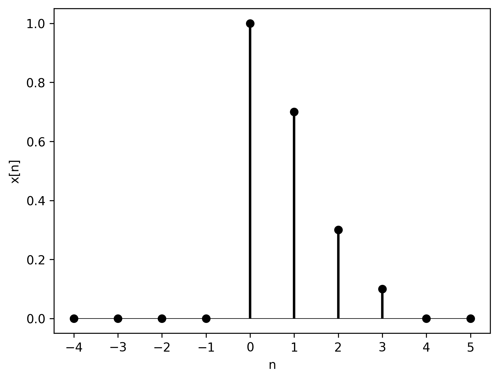Figure 1. $x[n]$.

and a discrete-time impulse delayed by 1 sample $h[n]$

Figure 2. $h[n]$.

The linear convolution between the two delays $x[n]$ by one sample, as expected

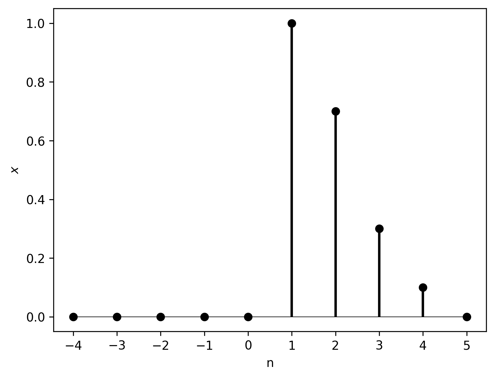Figure 3. Linear convolution between $x[n]$ and $h[n]$.

However, the circular convolution performs a circular shift of the signal $x[n]$

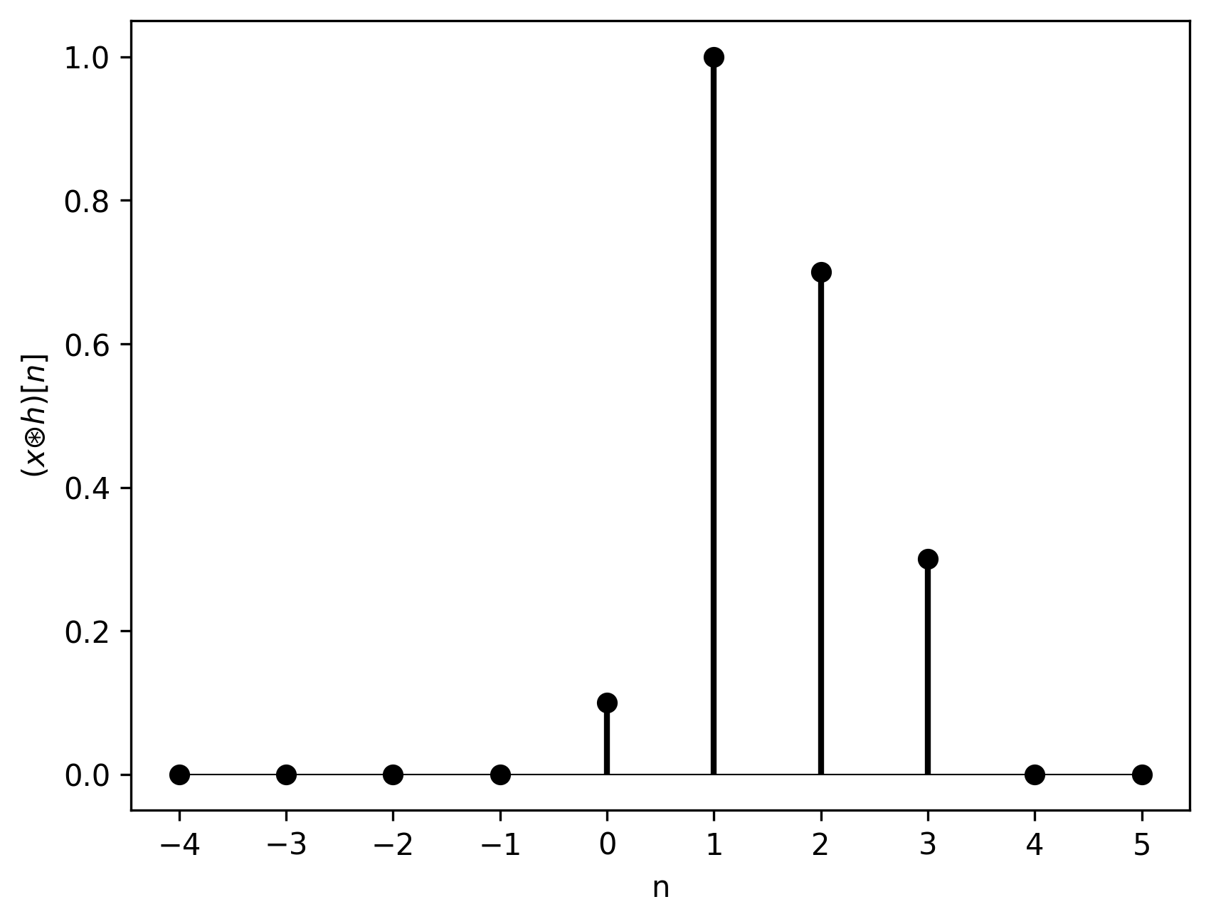Figure 4. Circular convolution between $x[n]$ and $h[n]$.

Circular shift means that whichever samples “fall off” one end reappear at the other end of the signal vector. In other words, the excessive samples “wrap around” the signal buffer.

Why Is the Convolution Circular?

The convolution property of the DFT results directly from the periodicity of the DFT.

The periodicity itself can be explained in at least two ways:

1. From the relation of the DFT to the discrete Fourier series (DFS).
2. From the sampling of the discrete-time Fourier transform around the unit circle on the z-plane.

Discrete Fourier Transform and Discrete Fourier Series

Discrete Fourier series is a representation of a periodic discrete signal $\tilde{x}[n]$ with period $N$ via a summation

$$\tilde{x}[n] = \frac{1}{N} \sum \limits_{k=0}^{N-1} \tilde{X}[k] e^{j(2\pi/N)kn}, \quad n \in \mathbb{Z}, \quad (8)$$

where

$$\tilde{X}[k] = \sum \limits_{n=0}^{N-1} \tilde{x}[n] e^{-j(2\pi/N)kn}, \quad n \in \mathbb{Z}. \quad (9)$$

Equation 9 is identical to Equation 1, i.e, the definition of the DFT, with the exception that the signal under the sum is periodic (denoted by the tilde) and $n$ is not bounded to the $\{0, \dots, N-1\}$ set. While the DFS assumes that the signal is periodic, i.e., it repeats itself modulo $N$, the DFT assumes that $x[n]$ is 0 for $n$ outside the $\{0, \dots, N-1\}$ index set [1].

The same holds for the DFT coefficients $X[k]$

$$X[k] = \begin{cases} \tilde{X}[k] \quad \text{if } k\in \{0, \dots, N-1\},\newline 0 \quad \text{otherwise}. \end{cases} \quad (10)$$

Unfortunately, the fact that $x[n]$ and $X[k]$ are 0 for $n,k \notin \{0, \dots, N-1\}$ is only implicit. It means we can state it but we cannot enforce it. Since the DFT uses directly the formulas of the DFS, the DFT will behave as if the signal $x[n]$ was periodic with period $N$. The only solution to that, would be padding the signal vector $x[n]$ with infinitely many zeros. Without such a padding, the DFT $X[k]$ is also periodic with period $N$.

DFT Periodicity Example

Let’s say we have a signal $x[n]$ given as a vector with four samples

Figure 5. $x[n]$.

You may think it is defined as follows

Figure 6. $x[n]$ as we wish it to be.

but the DFS (and the DFT accordingly) treat it as

Figure 7. $x[n]$ as seen by discrete Fourier series and the discrete Fourier transform.

Analogously, in the discrete frequency domain, we can obtain the magnitude Fourier coefficients $|X[k]|$ from Equation 1. This yields

Figure 8. Magnitude discrete-frequency coefficients of $x[n]$.

Again, one may assume that it is defined as follows

Figure 9. Magnitude DFT of $x[n]$ naively visualized with zeros surrounding the 4 nonzero coefficients.

but the inherent periodicity of the DFT results in

Figure 10. True magnitude DFT of $x[n]$.

Sampling of the Fourier transform

All of the above observations are confirmed when one treats the DFT as a sampled version of the band-limited discrete-time Fourier transform (DTFT). Discrete-time Fourier transform is the z-transform evaluated on the unit circle [2]. The DFT samples the DTFT at points fixed by the sampling rate. Since we sample around a circle, after $N$ samples we wrap around and start sampling the same points again. Refer to [1] for a more detailed explanation of this approach to DFT’s periodicity.

Aliasing in the Time Domain

Having established that the DFT is periodic, we can now explain the circular convolution phenomenon. I like to think of it as aliasing in the time domain.

Note: We have discussed the notion of aliasing in the frequency domain in one of the previous articles.

Output Length of Discrete Convolution

Let’s recall our signal $x[n]$ from Figure 1 and signal $h[n]$ from Figure 2. $x$ is of length 4, $h$ is of length 2. In Figure 3 we can see that the linear convolution between $x$ and $h$ is of length 5. In general, a convolution of two sequences of length $N$ and $M$ respectively yields a signal of length $N + M - 1$ [3].

How does it look when we go through the DFT domain?

Multiplication in the DFT domain

Adopting the notation from Equations 3 and 4, let’s denote by $Y[k]$ the multiplication of $x$’s and $h$’s DFTs

$$Y[k] = X[k]H[k] \quad k \in \{0, \dots, 3\}. \quad (11)$$

In order to make the index $k$ correspond to the same discrete frequencies for $X[k]$ and $H[k]$, discrete-frequency coefficients $X$ and $H$ need to be of equal length. We achieve it by padding $h$ with 2 zeros, i.e., replacing the 2-element signal $h$ with a 4-element one with values 0, 1, 0, 0 for $k=0,1,2,3$ respectively. Now $x$ and $h$ are of equal length and their DFTs are as well.

Back to the time domain

We now want to find signal $y[n]$ that corresponds to $Y[k]$, i.e.,

$$y[n] \stackrel{\mathcal{DFT}}{\longleftrightarrow} Y[k]. \quad (12)$$

We can achieve it via inverse discrete Fourier transform (iDFT)

$$y[n] = \mathcal{IDFT}\{Y[k]\} = \sum \limits_{k=0}^{N-1} Y[k] e^{j(2\pi/N)kn}. \quad (13)$$

If $x$ and $h$ were continuous-time and we were using the Fourier transform instead of the discrete Fourier transform, the convolution theorem would tell us that $y$ is the convolution of $x$ and $h$. We explicitly showed that the convolution of $x$ and $h$ should be a discrete signal of length 5 (see Figure 3). How long is $y$?

Inverse DFT inherently assumes that the time domain signal is of the same length as the frequency-domain coefficient vector. Thus, $y[n]$ is of length 4. So by multiplying frequency-domain vectors $\pmb{X}$ and $\pmb{H}$ and going back to the discrete-time domain we squashed a 5-element-long vector into a 4-element-long vector. Thus, we introduced aliasing in the time domain; hence the wrap-around of the last sample in Figure 4, and more broadly, circular convolution effect.

In mathematical terms,

$$y[n] = x[n] \circledast h[n]. \quad (14)$$

An Important Conclusion

We have seen that the circular convolution somehow distorts the linear convolution. But in our example, $x$ was circularly shifted, not completetely destroyed. Moreover, all but the first sample were valid samples of the linear convolution. Thus, we might suspect that sufficiently lengthening $\pmb{x}$ and $\pmb{h}$ with zero-padding would allow us to obtain the linear convolution out of the circular convolution result. This is the basis of fast convolution algorithms, which will be discussed in one of the following articles.

Circular vs. Linear Convolution

The conclusion from the previous section is that

A subset of the circular convolution result corresponds to the linear convolution result.

The question is: which subset?

Example: Common Samples of Linear and Circular Convolution

Figures 11 and 12 present the linear and circular convolution example, respectively, with marked matching samples. They match in terms of indices and amplitude.

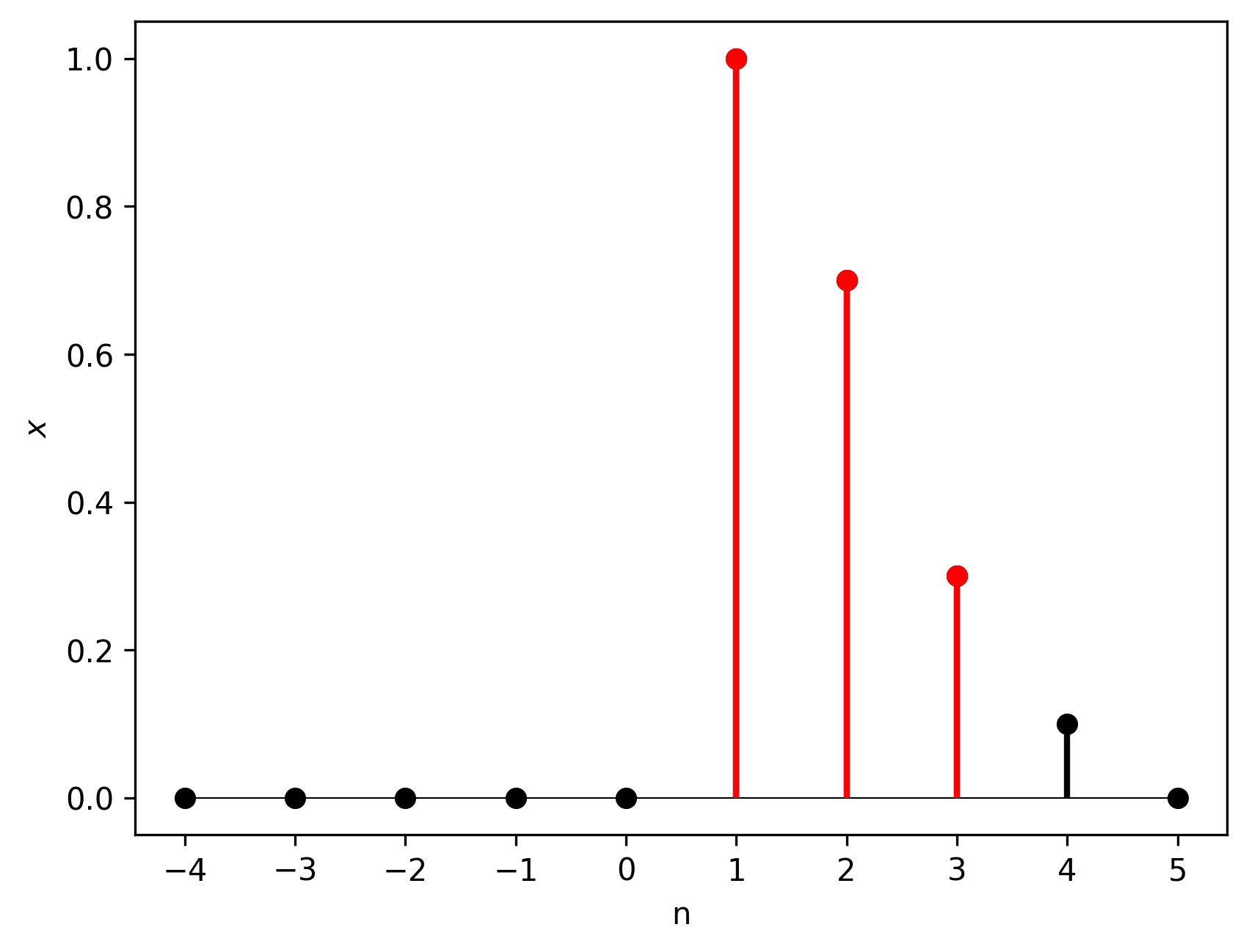Figure 11. Linear convolution result. Samples marked in red would also be correctly calculated by the circular convolution.

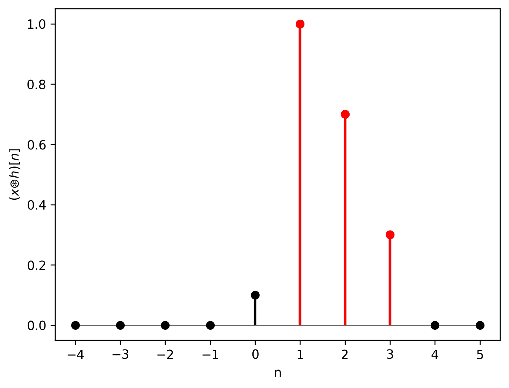Figure 12. Circular convolution result. Samples marked in red correspond to the linear convolution result in terms of index and amplitude.

To understand fully which samples in the circular convolution correspond to the correct samples of the linear convolution we need to look at a concept broader than circular convolution: periodic convolution.

Periodic Convolution

Circular convolution is an example of periodic convolution–a convolution of two periodic sample sequences (with the same period) evaluated over only one period [1]. It’s formula is identical to the formula of the circular convolution (Equation 6), but we assume that its output is periodic. “But in our case $x$ and $h$ are not periodic!”, you might say. Yes, they are not periodic, unless we compute their DFTs. The DFT assumes the signal to be perodic and, thus, going into the DFT domain introduces the periodicity permanently. It does not have to be harmful; on the contrary, it can be quite useful. It just requires us to be extra cautious.

Let’s compare the linear convolution and the periodic convolution. Given signals $x$ and (zero-padded) $h$, their periodic versions look as follows (black color indicates samples stored in the vector, grey color indicates implicit sample values)

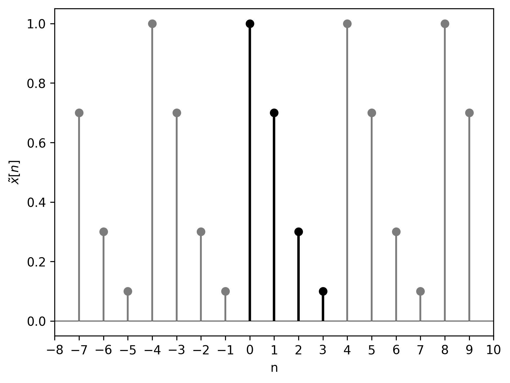Figure 13. Signal 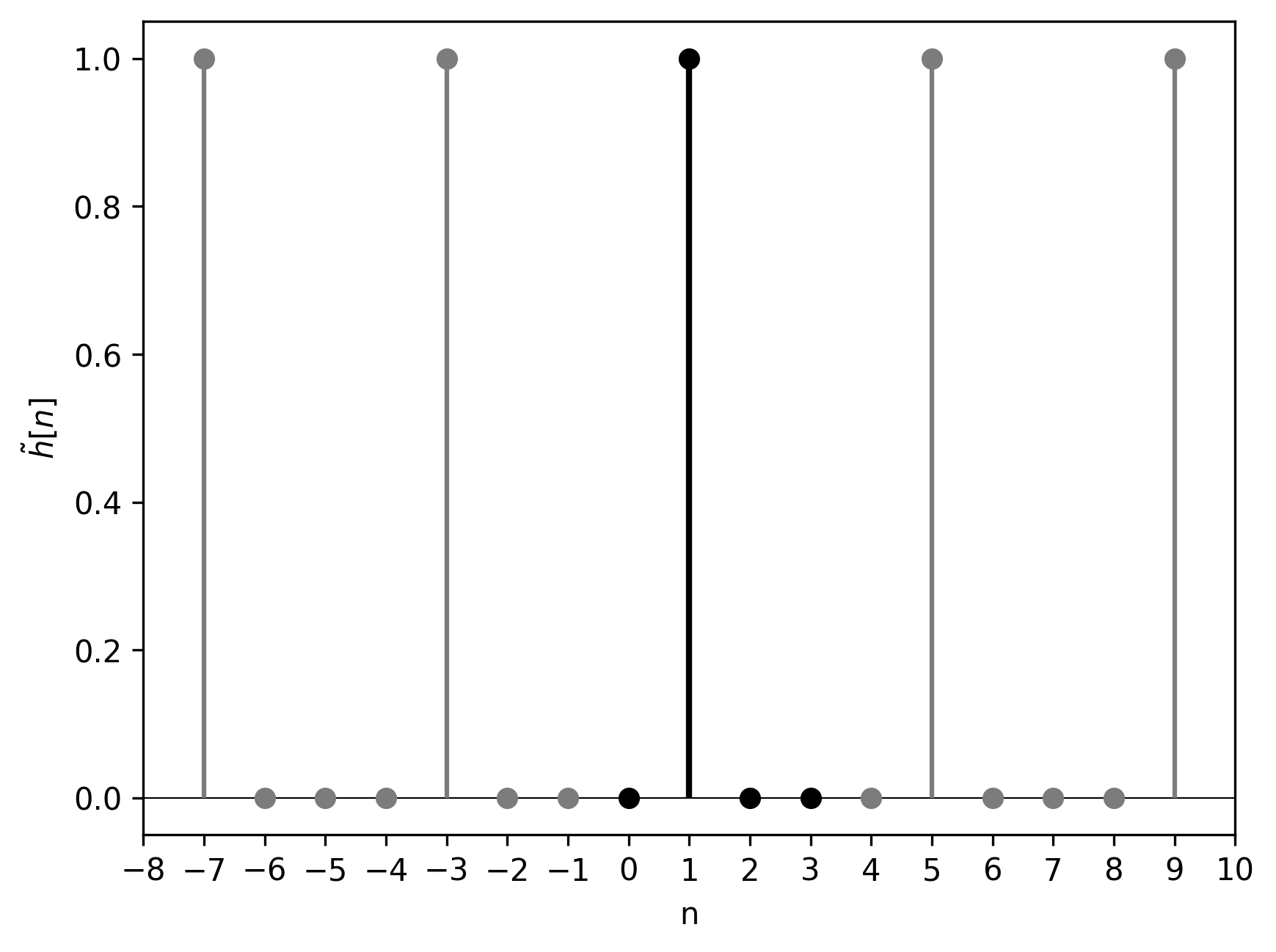$\tilde{x}$: periodic version of $x$. Figure 14. Signal $\tilde{h}$: periodic version of $h$.

Let’s compare the linear convolution of the original $x$ and $h$

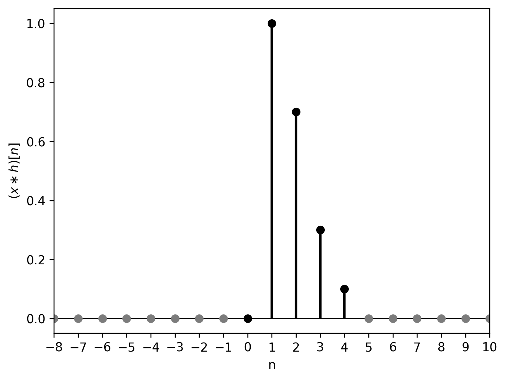Figure 15. Linear convolution of $x$ and $h$. Its length is 5.

with the periodic convolution of their periodic counterparts

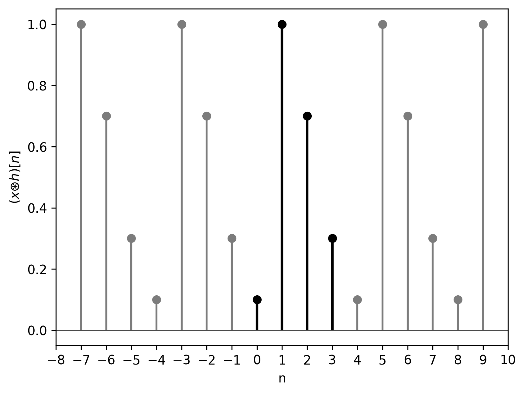Figure 16. Periodic convolution of $\tilde{x}$ and $\tilde{h}$. Its length is 4 and it’s periodic.

We can observe that the circular convolution is a superposition of the linear convolution shifted by 4 samples, i.e., 1 sample less than the linear convolution’s length. That is why the last sample is “eaten up”; it wraps around and is added to the initial 0 sample.

Once again: $x$ had length 4, $h$ had length 2, their linear convolution had length 5, the circular convolution had length 4, and the “valid” samples were the last 3. As we will see next the “excessive” sample wrapped around and “destroyed” the first sample, thus, we were left with only 3 samples that were identical to the linear convolution result. This is what I mean by “time-domain aliasing”: the periodic copies of the linear convolution (as implied by the DFT) start overlapping because we didn’t left them enough space (=“frequency-domain sampling rate”) in the DFT domain. Thus, we get time-domain artifacts.

Valid Samples of Circular Convolution: The Answer

Let’s summarize what we have discovered so far:

• Multiplication in the DFT domain is equivalent to circular convolution in the discrete-time domain.
• $N$-point DFT treats the signals as $N$-periodic.
• Linear convolution of discrete signals of length $M$ and $N$ has length $M+N-1$.
• $N$-point circular convolution has length $N$.

Let’s assume that we have two signals, of length $M$ and $N$, $M \geq N$. We want to know which samples of their circular convolution are equal to the corresponding samples of their linear convolution.

1. First, we pad the shorter signal with zeros. Now both signals have length $M$.
2. The result of the circular convolution has length $M$.
3. The samples that did not fit the linear convolution wrapped around and were added to the beginning of the output. The exact number of wrapped-around samples is $M + N - 1 - M = N - 1.$
4. The above means that the first $N-1$ samples of the output need to be discarded. This means that the last $M - N + 1$ samples are valid, i.e., samples at indices $\{N, N+1, \dots, M-1\}$ (we start indexing from 0).

Circular Convolution Implementation

A straightforward implementation of the circular convolution, as presented in Equation 6, is rather brute-force

import numpy as np

def periodic_convolution_naive(x, h):
    assert x.shape == h.shape, 'Inputs to periodic convolution '\
                               'must be of the same period, i.e., shape.'

    N = x.shape[0]

    output = np.zeros_like(x)

    for n in range(N):
        for m in range(N):
            output[n] += x[m] * h[(n - m) % N]
    
    return output

This implementation has time complexity $O(N^2)$.

However, the convolution property of the DFT, as presented in Equation 5, suggests a much more efficient implementation

import numpy as np

def periodic_convolution_fast(x, h):
    assert x.shape == h.shape, 'Inputs to periodic convolution '\
                               'must be of the same period, i.e., shape.'

    X = np.fft.fft(x)
    H = np.fft.fft(h)

    return np.real(np.fft.ifft(np.multiply(X, H)))

The complexity of the “fast” implementation is determined by the complexity of the forward and inverse DFT as implemented in the numpy.fft module, which is $O(N \log N)$.

Equal shapes checked in the assertion can be ensured by padding the shorter signal with zeros.

The efficient circular convolution implementation via the Fast Fourier Transform (FFT) will serve as a basis when we will discuss fast linear convolution implementations.

Summary

In this article, we looked at the difference between the circular and the linear convolution. The former treats both given sequences as periodic and is evaluated only for the number of samples corresponding to the period.

A subset of samples resulting from the circular convolution corresponds to the samples of the linear convolution.

Circular convolution can be implemented efficiently via multiplication in the DFT domain.

Bibliography

[1] Alan V Oppenheim, Ronald W. Schafer Discrete-Time Signal Processing, 3rd Edition, Pearson 2010.

[2] Alan V. Oppenheim, Alan S. Willsky, with S. Hamid Signals and Systems, 2nd Edition, Pearson 1997.

[3] Frank Wefers Partitioned convolution algorithms for real-time auralization, PhD Thesis, Zugl.: Aachen, Techn. Hochsch., 2015.