Sine, Saw, Square, Triangle, Pulse: Basic Waveforms in Synthesis and Their Properties

Read this to use their full potential and avoid any caveats!

A waveform is a graphical representation of a wave.

Sound synthesis is based on 5 waveforms: the sine, the triangle, the sawtooth (saw), the pulse, and the square (which is a particular case of the pulse).

To use them effectively in sound synthesis compositions or audio programming, you need to know their basic properties:

• mathematical formula to generate it,
• time-domain visualization,
• amplitude spectrum: which harmonics are present and how their amplitudes decay, and
• how it sounds!

In this article, you will learn all these properties about the 5 basic waveforms.

Note: this article shows the waveforms in their continuous (analog) form, which means that issues such as aliasing or efficient generation are not considered. Keep in mind that all of these waveforms (apart from the sine) have an infinite amplitude spectrum.

Why Learn About Basic Waveforms?

Learning about basic waveforms in sound synthesis will help you

• exploit the capabilities of modern synthesizers,
• achieve the desired timbre even during live performances,
• understand the behavior of oscillators (often marked as VCO, voltage-controlled oscillator) and modulators (often marked as LFO, low-frequency oscillator),
• employ these waveforms in mathematical derivations of analysis, synthesis, and audio effects,
• write efficient code to generate these waveforms for sound synthesis and audio effects algorithms,
• detect any inconsistencies in these signals in a system,
• avoid potential issues with aliasing, and
• discover where aliasing may come from (e.g., from an unbounded spectrum).

The Waveforms

Jump to the Waveform of Choice

1. Sine
2. Triangle
3. Square
4. Sawtooth (Saw)
5. Pulse

Sine

The sine is the most basic of sound synthesis waveforms.

The sine formula is simple

$s(t) = \sin (2 \pi f t), \quad (1)$

where $f$ is the frequency of the sine in Hz and $t$ is time in seconds.

A sine at 220 Hz sounds like this:

The time-domain representation (waveform) of the sine looks like this:

Figure 1. Sine waveform: time-domain representation of the sine wave.

The amplitude spectrum of a sine is very boring because it consists of just one partial: the fundamental frequency.

Figure 2. Amplitude spectrum of a sine.

As you can see, it has only one harmonic. That makes sense because spectrum calculation assumes that the analyzed signal is a superposition (a sum) of sines. And one sine consists of just… one sine 🙃

Triangle

A triangle is just a little bit more complicated than the sine.

The triangle formula is [Wikipedia]

$s(t) = 4 \left| ft - \left\lfloor ft + \frac{1}{2} \right\rfloor \right| - 1, \quad (2)$

where $f$ is the triangle’s frequency in Hz and $t$ is time in seconds.

A triangle wave at 220 Hz sounds like this:

As you can hear, it’s a bit brighter than the sine.

The triangle waveform in the time-domain looks as follows.

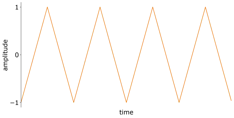Figure 3. Triangle waveform: time-domain representation of the triangle wave.

The plot in Figure 3 indeed looks like a triangle.

This makes the formula from Equation 2 more intuitive: a triangle waveform is, in essence, the difference between a linear function and a shifted step function. This difference increases and decreases piecewise linearly and so we obtain a triangle.

The amplitude spectrum of the triangle waveform contains only odd harmonics (Figure 4).

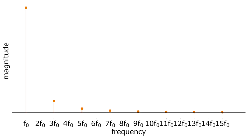Figure 4. Amplitude spectrum of a triangle.

The amplitudes of the harmonics decay as $\frac{1}{n^2}$, where $n$ is the harmonic’s index (the fundamental has $n=1$, the first overtone has $n=2$, and so on).

Square

The square wave is more interesting than the sine or the triangle because of its characteristic, “empty” timbre.

The square wave at 220 Hz sounds like this:

For me, the simplest formula for the square waveform is just taking the sign of the sine:

$s(t) = \text{sgn} (\sin (2 \pi f t)), \quad (3)$

where $f$ is the square’s frequency in Hz and $t$ is time in seconds.

Of course, alternative formulas are possible, like ones using the modulo operation.

The square waveform in the time-domain has a rectangular shape (Figure 5).

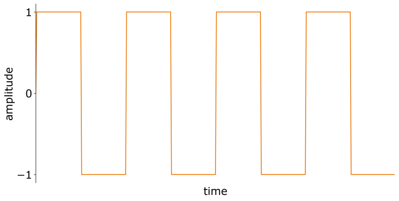Figure 5. Square waveform: time-domain representation of the square wave.

The amplitude spectrum of the square wave consists of only odd harmonics, exactly as was the case for the triangle (Figure 6).

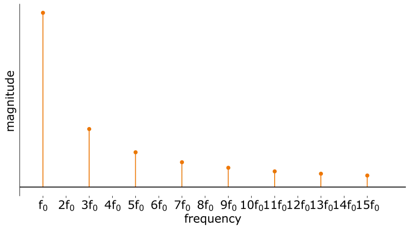Figure 6. Amplitude spectrum of a square.

The amplitudes of square’s harmonics decay slower than in the case of the triangle: they decay as $\frac{1}{n}$, where $n$ is the harmonic’s index ($n=1$ corresponds to the fundamental).

Sawtooth (Saw)

The sawtooth (or simply “saw”) waveform is my favorite waveform, thanks to its rich, “fat” sound that plays incredibly well with a good low-pass filter.

The sawtooth wave at 220 Hz sounds like this:

Ah, that’s so beautiful ❤️

The simplest formula for the sawtooth wave is a modulo approach:

$s(t) = 2 \left( t \% \frac{1}{f} \right) f - 1, \quad (0)$

where $f$ is the sawtooth’s frequency in Hz, $t$ is time in seconds, and $\%$ is the modulo operator applied to real values.

The formula reads, “increase the value linearly ($t$), jump back to 0 every period ($\% \frac{1}{f}$), scale to the $[0, 1]$ range (multiplication by $f$), and then expand the range from $[0, 1]$ to $[-1, 1]$ (multiplication by $2$ and subtraction of $1$).”

The sawtooth waveform in the time domain is shown in Figure 7.

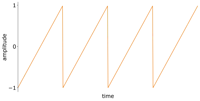Figure 7. Sawtooth waveform: time-domain representation of the sawtooth wave.

This is the so-called ramp-up sawtooth because its slope is rising within each period. Should it be falling, it would be called ramp-down sawtooth. Since it’s just a matter of phase inversion, ramp-up and ramp-down variants have the same properties. The slope matters the most when we use the sawtooth waveform to modulate some other parameter, i.e., when we use the sawtooth in a low-frequency oscillator (LFO). Then we can create a periodically rising sensation (ramp-up) or periodically falling (ramp-down).

The name “saw” comes from the teeth-like shape of the waveform.

The amplitude spectrum of the sawtooth can be seen in Figure 8.

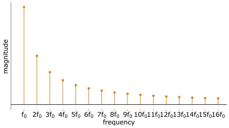Figure 8. Amplitude spectrum of a sawtooth.

The spectrum of the sawtooth waveform contains odd and even harmonics. The amplitudes of sawtooth’s harmonics decay as $\frac{1}{n}$, where $n$ is the harmonic’s index ($n=1$ corresponds to the fundamental frequency).

Pulse

The pulse waveform (also called a pulse train) is a generalization of the square waveform.

An example pulse waveform in the time domain is shown in Figure 9.

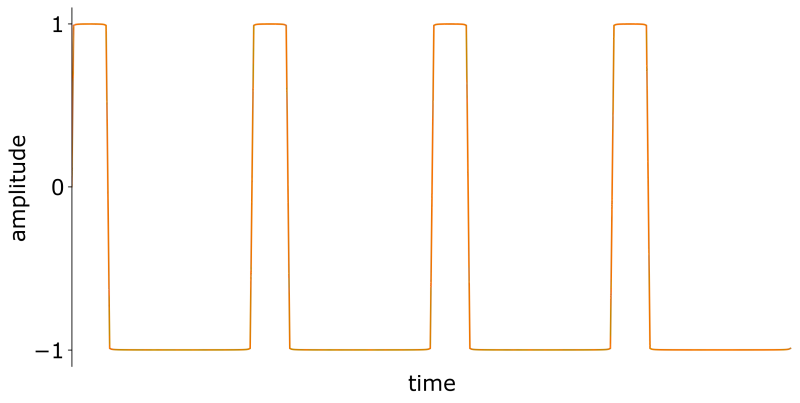Figure 9. Pulse waveform: time-domain representation of the pulse wave with 20% duty cycle.

This waveform’s duty cycle is 20%. It means that for 20% of its period, the value is 1. For the remaining 80%, the value is -1.

Duty cycle specifies for which fraction of the period the value of the waveform is 1.

For $D=0.5$, we obtain the square waveform.

The pulse waveform with 20% duty cycle at 220 Hz sounds like this:

The pulse wave could be generated in various ways. I used a Fourier series-based formula [Pluta2019]

$s(t) = (2D - 1) + \sum_{k=1}^{\infty} \frac{4}{k\pi} \sin (\pi k D) \cos (2 \pi k f_0 t - \pi k D), 10$

where $D$ is the duty cycle, $k$ is the harmonic’s index, $f_0$ is the fundamental frequency in Hz, and $t$ is time in seconds.

The amplitude spectrum of the pulse wave for $D=0.2$ case is shown in Figure 10.

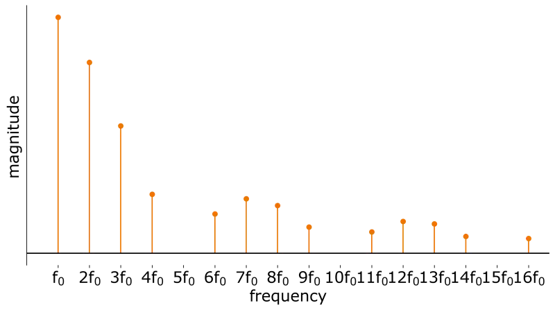Figure 11. Amplitude spectrum of a pulse wave with 20% duty cycle.

However, the amplitude spectrum changes dynamically with the duty cycle. I have visualized it on Figure 11.

Figure 12. Time-domain waveform and the amplitude spectrum of a pulse wave for different values of the duty cycle.

As you can see in the figure, for duty cycle equal to 50% we get the square wave and its odd-harmonics-only amplitude spectrum.

The first dip from the left in the amplitude spectrum is determined by the duty cycle: the dip occurs at the $D^{-1}$-th harmonic.

For example, for the square wave, $D=0.5$ so the first dip occurs at the $\left(\frac{1}{2}\right)^{-1} = 2$-nd harmonic.

In the figure, you can also see a small glitch around the DC (0 Hz) frequency. That is because for very high or very low values of the duty cycle, the DC component is pretty significant (the mean of the waveform’s values is significantly nonzero). I have deliberately hidden the DC component from the plots for clarity but some of it is still present because of the spectral leakage.

The DC component must be kept in mind in musical applications because it adds no musical information (we cannot hear it) but it can damage the hardware that it runs through.

Summary

In this article, you learned everything about the basic waveforms (sine, triangle, square, saw, pulse) that you need for sound synthesis. Being familiar with these waveforms will help you in exploiting synthesizers’ capabilities and coding your own.

These waveforms are one piece of the puzzle when it comes to developing your own software sound synthesizers. If you want to know what other information is necessary to develop audio plugins, download my free Ultimate Audio Plugin Developer Checklist.

Bibliography

[Pluta2019] Marek Pluta, Sound Synthesis for Music Reproduction and Performance, monograph, AGH University of Science and Technology Press, Kraków 2019.

[VälimäkiHuovilainen2006] Vesa Välimäki and Antti Huovilainen, Oscillator and Filter Algorithms for Virtual Analog Synthesis, Computer Music Journal, 30:2, pp. 19–31, Summer 2006. PDF

[Wikipedia] Triangle wave on Wikipedia. Access: 28.06.2022.